def doc_theme():
    return theme_minimal() + theme(
        panel_grid_minor=element_line(color="gray", linetype="--"),
)Simulating Halo, Cluster and Member Catalogs
Purpose
This tutorial shows how to generate mock halo/cluster catalogs and their galaxy members entirely from NumCosmo’s C objects, and how to chain them together with the MockPipeline orchestrator.
The generation is split into small, reusable pieces, each assembled from the existing modelling machinery rather than reimplemented:
NcHaloCatalogGeneratordraws a Poisson realization of the cluster number counts from aNcClusterAbundance, samples the observed redshift and mass through the cluster proxies, and (optionally) adds sky positions over anNcmSkyFootprintand the spherical-overdensity radiusr_Delta;NcGalaxyHODZheng07is a halo occupation distribution turning a halo mass into central and satellite galaxy counts;NcHaloCatalogMemberGeneratorpopulates each host with its galaxies, placing them in 3D withinr_Deltaand projecting them to sky coordinates and redshift;MockPipelinewires the cluster and member generators together and returns the two linkedNcHaloCatalogtables.
The resulting catalogs are ready to feed the matching tools of the Sky Match tutorial or the cluster number-counts likelihood.
Defining the Models
We start with a flat \(\Lambda\)CDM cosmology and the ingredients of the halo mass function: a linear matter power spectrum, a top-hat variance filter and a multiplicity function (NcMultiplicityFuncBocquet) with a critical \(\Delta = 200\) mass definition. The mass definition carried here is what fixes the meaning of r_Delta later on.
import numpy as np
import pandas as pd
import matplotlib.pyplot as plt
from IPython.display import HTML

from numcosmo_py import Nc, Ncm
from numcosmo_py.catalog import MockPipeline, catalog_to_table

Ncm.cfg_init()


def show_table(table, float_format="%.3f", max_rows=10):
    """Render an astropy Table as a compact HTML table."""
    return HTML(table.to_pandas().to_html(float_format=float_format, max_rows=max_rows))


cosmo = Nc.HICosmoDEXcdm.new()
cosmo.add_submodel(Nc.HIReionCamb.new())
cosmo.add_submodel(Nc.HIPrimPowerLaw.new())
cosmo["H0"] = 70.0
cosmo["Omegab"] = 0.05
cosmo["Omegac"] = 0.25
cosmo["Omegax"] = 0.70
cosmo["w"] = -1.0

dist = Nc.Distance.new(2.0)
psml = Nc.PowspecMLTransfer.new(Nc.TransferFuncEH())
psml.require_kmin(1.0e-3)
psml.require_kmax(1.0e3)
psf = Ncm.PowspecFilter.new(psml, Ncm.PowspecFilterType.TOPHAT)
psf.set_best_lnr0()

mulf = Nc.MultiplicityFuncBocquet.new()
mulf.set_mdef(Nc.MultiplicityFuncMassDef.CRITICAL)
mulf.set_Delta(200.0)
mulf.set_sim(Nc.MultiplicityFuncBocquetSim.DM)

hmf = Nc.HaloMassFunction.new(dist, psf, mulf)
hmf.prepare(cosmo)
Observable Proxies and Abundance
The cluster abundance needs proxies relating the true mass and redshift to the observed ones. We use a log-normal mass proxy (NcClusterMassLnnormal) and a global Gaussian photometric redshift (NcClusterPhotozGaussGlobal), and we collect every model into an NcmMSet.
cluster_m = Nc.ClusterMassLnnormal(
    lnMobs_min=np.log(1.0e14), lnMobs_max=np.log(1.0e16)
)
cluster_m["bias"] = 0.0
cluster_m["sigma"] = 0.2

cluster_z = Nc.ClusterPhotozGaussGlobal(
    pz_min=0.0, pz_max=0.7, z_bias=0.0, sigma0=0.03
)

cad = Nc.ClusterAbundance.new(hmf, None)

mset = Ncm.MSet.new_array([cosmo, cluster_z, cluster_m])
Footprint and Halo Occupation
The footprint (NcmSkyFootprintRectangular) is the sky region over which positions are drawn; the HOD turns each halo mass into a number of central and satellite galaxies.
footprint = Ncm.SkyFootprintRectangular.new(10.0, 14.0, -2.0, 2.0)

cad.set_area(footprint.get_area())
cad.prepare(cosmo, cluster_z, cluster_m)

hod = Nc.GalaxyHODZheng07.new()
Generating the Mock
MockPipeline assembles the cluster generator (with the footprint and radius enabled) and the member generator, so a single call produces both catalogs.
pipeline = MockPipeline(cad, hod, footprint)

rng = Ncm.RNG.seeded_new(None, 1)
mock = pipeline.generate(mset, rng)

clusters = mock.clusters
members = mock.members

print(f"Generated {len(clusters)} clusters and {len(members)} members.")
Generated 239 clusters and 864 members.The cluster catalog carries the true and observed redshift/mass, the sky position and the spherical-overdensity radius r_Delta, plus a cluster_id join key:
Code
show_table(clusters)| z_true | lnM_true | z_obs_0 | lnM_obs_0 | ra | dec | r_Delta | cluster_id | |
|---|---|---|---|---|---|---|---|---|
| 0 | 0.319 | 32.252 | 0.285 | 32.240 | 12.480 | -1.182 | 0.863 | 0 |
| 1 | 0.501 | 32.648 | 0.434 | 32.796 | 13.796 | 1.025 | 0.917 | 1 |
| 2 | 0.545 | 32.505 | 0.537 | 32.480 | 12.417 | -1.332 | 0.860 | 2 |
| 3 | 0.245 | 32.591 | 0.244 | 32.886 | 13.194 | -0.615 | 0.993 | 3 |
| 4 | 0.598 | 33.060 | 0.607 | 33.123 | 12.299 | -1.162 | 1.013 | 4 |
| ... | ... | ... | ... | ... | ... | ... | ... | ... |
| 234 | 0.573 | 32.551 | 0.643 | 32.309 | 10.630 | 0.659 | 0.864 | 234 |
| 235 | 0.357 | 32.464 | 0.353 | 32.497 | 12.005 | -0.951 | 0.913 | 235 |
| 236 | 0.059 | 33.351 | 0.056 | 33.245 | 12.139 | 0.664 | 1.363 | 236 |
| 237 | 0.633 | 32.116 | 0.578 | 32.409 | 10.029 | -0.122 | 0.729 | 237 |
| 238 | 0.702 | 32.232 | 0.667 | 32.473 | 11.605 | 1.370 | 0.738 | 238 |
Each member links back to its host cluster through parent_id, which matches the cluster_id column of the cluster table:
Code
show_table(members)| galaxy_id | parent_id | is_central | ra | dec | z | |
|---|---|---|---|---|---|---|
| 0 | 0 | 0 | True | 12.480 | -1.182 | 0.319 |
| 1 | 1 | 0 | False | 12.445 | -1.203 | 0.319 |
| 2 | 2 | 1 | True | 13.796 | 1.025 | 0.501 |
| 3 | 3 | 1 | False | 13.786 | 1.003 | 0.501 |
| 4 | 4 | 1 | False | 13.801 | 1.047 | 0.501 |
| ... | ... | ... | ... | ... | ... | ... |
| 859 | 859 | 236 | False | 12.161 | 0.487 | 0.059 |
| 860 | 860 | 236 | False | 12.247 | 0.581 | 0.059 |
| 861 | 861 | 236 | False | 12.265 | 0.661 | 0.059 |
| 862 | 862 | 237 | True | 10.029 | -0.122 | 0.633 |
| 863 | 863 | 238 | True | 11.605 | 1.370 | 0.702 |
n_central = int(np.sum(members["is_central"]))
print(f"{n_central} centrals and {len(members) - n_central} satellites.")
239 centrals and 625 satellites.Visualising the Catalogs
The clusters trace the footprint; member galaxies cluster tightly around their hosts. We size the cluster markers by mass and colour them by redshift.
fig, ax = plt.subplots(figsize=(7, 6))

ax.scatter(members["ra"], members["dec"], s=2, color="0.7", label="members")
sc = ax.scatter(
    clusters["ra"],
    clusters["dec"],
    s=8 + 6 * (clusters["lnM_true"] - clusters["lnM_true"].min()),
    c=clusters["z_true"],
    cmap="viridis",
    edgecolor="k",
    linewidth=0.3,
    label="clusters",
)
fig.colorbar(sc, ax=ax, label="cluster $z$")
ax.set_xlabel("RA [deg]")
ax.set_ylabel("Dec [deg]")
ax.legend(loc="upper right")
plt.show()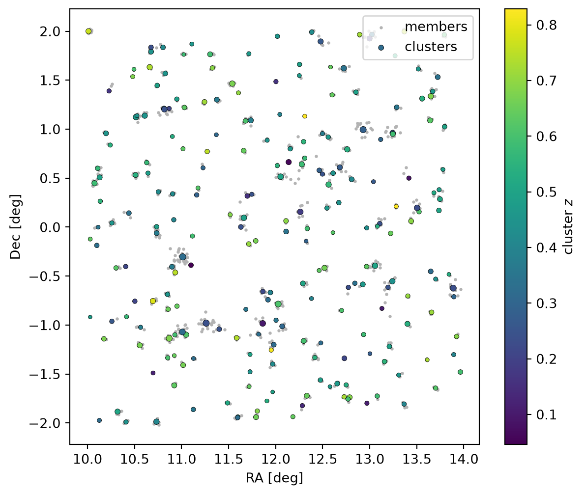
Zooming on the most massive cluster shows the members distributed around the host position, with the central sitting exactly on it.
i = int(np.argmax(clusters["lnM_true"]))
cid = int(clusters["cluster_id"][i])
sel = members[members["parent_id"] == cid]
is_cen = np.asarray(sel["is_central"], dtype=bool)

fig, ax = plt.subplots(figsize=(5, 5))
ax.scatter(sel["ra"][~is_cen], sel["dec"][~is_cen], s=12, label="satellites")
ax.scatter(sel["ra"][is_cen], sel["dec"][is_cen], s=80, marker="*",
           color="crimson", label="central")
ax.scatter(clusters["ra"][i], clusters["dec"][i], s=120, facecolor="none",
           edgecolor="k", label="host")
ax.set_xlabel("RA [deg]")
ax.set_ylabel("Dec [deg]")
ax.legend()
ax.set_title(f"Members of cluster {cid}")
plt.show()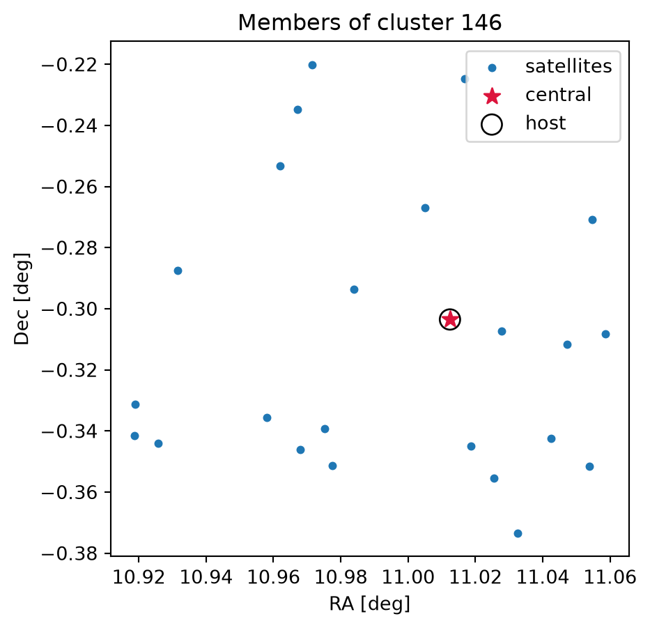
Working with the Generators Directly
MockPipeline is a thin wrapper; the underlying generators can be used on their own. For example, to obtain just the cluster catalog with positions and radius, enable them with nc_halo_catalog_generator_set_footprint and nc_halo_catalog_generator_set_with_radius:
cluster_gen = Nc.HaloCatalogGenerator.new(cad)
cluster_gen.set_footprint(footprint)
cluster_gen.set_with_radius(True)

hcat = cluster_gen.generate(mset, Ncm.RNG.seeded_new(None, 2))
print(list(hcat.peek_columns()))
['z_true', 'lnM_true', 'z_obs_0', 'lnM_obs_0', 'ra', 'dec', 'r_Delta']Code
show_table(catalog_to_table(hcat))| z_true | lnM_true | z_obs_0 | lnM_obs_0 | ra | dec | r_Delta | |
|---|---|---|---|---|---|---|---|
| 0 | 0.560 | 32.346 | 0.591 | 32.251 | 11.747 | 1.237 | 0.811 |
| 1 | 0.617 | 32.779 | 0.627 | 32.749 | 13.403 | 1.291 | 0.915 |
| 2 | 0.295 | 32.178 | 0.324 | 32.240 | 11.957 | 0.146 | 0.849 |
| 3 | 0.556 | 32.280 | 0.547 | 32.262 | 10.881 | -0.045 | 0.794 |
| 4 | 0.645 | 32.431 | 0.641 | 32.541 | 10.111 | -0.633 | 0.806 |
| ... | ... | ... | ... | ... | ... | ... | ... |
| 244 | 0.688 | 32.351 | 0.691 | 32.261 | 12.477 | 0.331 | 0.771 |
| 245 | 0.594 | 32.311 | 0.648 | 32.265 | 13.552 | 1.552 | 0.790 |
| 246 | 0.627 | 32.218 | 0.671 | 32.307 | 11.621 | -1.219 | 0.756 |
| 247 | 0.587 | 32.825 | 0.536 | 32.854 | 12.574 | 1.978 | 0.941 |
| 248 | 0.584 | 32.353 | 0.653 | 32.367 | 13.869 | -1.642 | 0.805 |
The member generator can then populate any host catalog carrying the ra, dec, z_true, lnM_true and r_Delta columns, via nc_halo_catalog_member_generator_generate:
member_gen = Nc.HaloCatalogMemberGenerator.new(hod)
member_hcat = member_gen.generate(hcat, mset, Ncm.RNG.seeded_new(None, 3))
print(f"{member_hcat.len()} members generated.")
850 members generated.Summary
We generated a linked cluster and member mock entirely from NumCosmo C objects: the cluster abundance and proxies produce the cluster catalog, a halo occupation distribution populates each cluster with galaxies, and MockPipeline returns both as astropy tables linked by id. These catalogs feed naturally into the Sky Match tools and the cluster number-counts likelihood.
API Reference
The objects used in this tutorial:
- catalogs:
NcHaloCatalog,NcmCatalog - generators:
NcHaloCatalogGenerator(nc_halo_catalog_generator_set_footprint,nc_halo_catalog_generator_set_with_radius,nc_halo_catalog_generator_generate) andNcHaloCatalogMemberGenerator(nc_halo_catalog_member_generator_generate) - occupation:
NcGalaxyHOD,NcGalaxyHODZheng07 - footprint:
NcmSkyFootprint,NcmSkyFootprintRectangular - abundance and proxies:
NcClusterAbundance,NcClusterMassLnnormal,NcClusterPhotozGaussGlobal
The Python-level helpers MockPipeline and catalog_to_table live in the numcosmo_py.catalog subpackage.