def doc_theme():
    return theme_minimal() + theme(
        panel_grid_minor=element_line(color="gray", linetype="--"),
)Matching Observations to Simulations
Purpose
This document provides a guide to using NumCosmo’s sky_match module, which employs the SkyMatch class to match objects in the sky.
The SkyMatch class is designed to associate detected objects, such as galaxy clusters or halos, with observational data. A common application is matching cluster detections to halos in simulations. This process enables the evaluation of completeness and purity in observations.
In this tutorial, we generate mock data for galaxy clusters and halos, then use the SkyMatch class to perform matching and analyze the results.
Defining Theoretical Models
Cosmological Model
To begin, we define a cosmological model using NumCosmo’s background cosmology models. We also create an Nc.Distance object to compute the cosmological distances required for the weak lensing analysis.
For this example, we consider a Lambda Cold Dark Matter (\(\Lambda\)CDM) cosmology with the following parameters:
- \(\Omega_{c0} = 0.25\): Cold dark matter density parameter at present
- \(\Omega_{b0} = 0.05\): Baryon density parameter at present
- \(\Omega_{k0} = 0\): Curvature density parameter at present
- \(H_0 = 70.0\): Hubble constant in km/s/Mpc
import numpy as np
import pandas as pd
import matplotlib.pyplot as plt
from astropy.table import Table
import pandas as pd
from IPython.display import HTML

from numcosmo_py import Nc, Ncm
from numcosmo_py.catalog import (
    BestCandidates,
    Coordinates,
    DistanceMethod,
    SelectionCriteria,
    SkyMatch,
    SkyMatchResult,
)

Ncm.cfg_init()

Omega_b = 0.05
Omega_c = 0.25
Omega_k = 0.0
H0 = 70.0

# Create a cosmology object
cosmo = Nc.HICosmoDEXcdm.new()
cosmo.omega_x2omega_k()
cosmo["Omegab"] = Omega_b
cosmo["Omegac"] = Omega_c
cosmo["Omegak"] = Omega_k
cosmo["H0"] = H0
cosmo["w"] = -1.0

dist = Nc.Distance.new(100.0)
dist.compute_inv_comoving(True)
dist.prepare(cosmo)

# Lets fix the numpy seed to get reproducible results
np.random.seed(74682)
Generating Mock Data
To illustrate the matching process, we generate simulated mock data for galaxy clusters and halos.
While these configurations do not represent typical observational distributions, they are chosen to ensure the figures remain clear and readable.
We use a simple random distribution to assign positions, redshifts, and masses to both clusters and halos:
- Positions:
- Defined by right ascension (RA) and declination (Dec) in degrees.
- RA is uniformly sampled in the range \([-10^\circ, 10^\circ]\).
- Dec is sampled uniformly in \(\sin(\text{Dec})\) and converted back to degrees to ensure uniform coverage on the sphere.
- Defined by right ascension (RA) and declination (Dec) in degrees.
- Redshifts:
- Uniformly distributed between 0.2 and 0.5.
- Masses:
- Sampled uniformly in \(\log_{10} M_{\odot}\) within the range \([13, 15]\).
- The additional 100 halos are sampled uniformly in \(\log_{10} M_{\odot}\) within the range \([10, 13]\).
To demonstrate the matching process, we generate:
- 100 galaxy clusters, each with assigned positions, redshifts, and masses.
- 200 halos, with two different placement strategies:
- First 100 halos are placed within 5 Mpc of a cluster’s position (in each dimension), simulating a correlated distribution.
- Remaining 100 halos are distributed randomly to provide a broader test case.
- First 100 halos are placed within 5 Mpc of a cluster’s position (in each dimension), simulating a correlated distribution.
This setup ensures that some halos are closely associated with clusters, while others are randomly placed to create a more comprehensive matching scenario.
# Constants
CLUSTER_LENGTH = 100
HALO_LENGTH = 200

RA_MIN, RA_MAX = -10.0, 10.0
DEC_MIN, DEC_MAX = -10.0, 10.0
Z_MIN, Z_MAX = 0.2, 0.5
LOGM_MIN, LOGM_MAX = 13.0, 15.0  # Mass in log10 solar masses
LOGM_ADD_HALO_MIN, LOGM_ADD_HALO_MAX = 10.0, 13.0

# Generate cluster positions, redshifts, and masses
cluster_ra = np.random.uniform(RA_MIN, RA_MAX, CLUSTER_LENGTH)
cluster_sin_dec = np.random.uniform(
    np.sin(np.radians(DEC_MIN)), np.sin(np.radians(DEC_MAX)), CLUSTER_LENGTH
)
cluster_dec = np.degrees(np.arcsin(cluster_sin_dec))
cluster_z = np.random.uniform(Z_MIN, Z_MAX, CLUSTER_LENGTH)
cluster_logm = np.random.uniform(LOGM_MIN, LOGM_MAX, CLUSTER_LENGTH)
# Let's compute the cluster radii, and the 3D positions
cluster_r = np.array(dist.comoving_array(cosmo, cluster_z)) * cosmo.RH_Mpc()
cluster_x1 = (
    cluster_r * np.cos(np.radians(cluster_dec)) * np.cos(np.radians(cluster_ra))
)
cluster_x2 = (
    cluster_r * np.cos(np.radians(cluster_dec)) * np.sin(np.radians(cluster_ra))
)
cluster_x3 = cluster_r * np.sin(np.radians(cluster_dec))

# Generate halo positions, redshifts, and masses
# Lets first sample a halo < 5.0 Mpc from the cluster in each dimension
D_DIM = 5.0

halo_x1 = cluster_x1 + np.random.uniform(-D_DIM, D_DIM, CLUSTER_LENGTH)
halo_x2 = cluster_x2 + np.random.uniform(-D_DIM, D_DIM, CLUSTER_LENGTH)
halo_x3 = cluster_x3 + np.random.uniform(-D_DIM, D_DIM, CLUSTER_LENGTH)
halo_ra = np.degrees(np.arctan2(halo_x2, halo_x1))
halo_dec = np.degrees(np.arcsin(halo_x3 / cluster_r))
halo_r = np.sqrt(halo_x1**2 + halo_x2**2 + halo_x3**2)
halo_z = [dist.inv_comoving(cosmo, r / cosmo.RH_Mpc()) for r in halo_r]

# Now for the halo masses we use the cluster's masses added a Gaussian noise
halo_logm = cluster_logm + np.random.normal(0, 1.0, CLUSTER_LENGTH)

# Finally we add 100 more halos randomly
DELTA_OBJECTS = HALO_LENGTH - CLUSTER_LENGTH
halo_ra = np.append(halo_ra, np.random.uniform(RA_MIN, RA_MAX, DELTA_OBJECTS))
halo_dec = np.append(halo_dec, np.random.uniform(DEC_MIN, DEC_MAX, DELTA_OBJECTS))
halo_z = np.append(halo_z, np.random.uniform(Z_MIN, Z_MAX, DELTA_OBJECTS))
halo_logm = np.append(
    halo_logm, np.random.uniform(LOGM_ADD_HALO_MIN, LOGM_ADD_HALO_MAX, DELTA_OBJECTS)
)
Visualizing Cluster and Halo Distributions
We plot the generated cluster and halo positions, with the dot sizes proportional to the object’s \(\log_{10} M_{\odot}\).
Code
# Scale marker sizes with log mass
def scale_marker_size(log_mass, base_size=20, scale_factor=30):
    arr = scale_factor * (log_mass - LOGM_MIN)
    return base_size + np.where(arr < 0, 0, arr)


cluster_sizes = scale_marker_size(cluster_logm)
halo_sizes = scale_marker_size(halo_logm)

fig, ax = plt.subplots(figsize=(10, 8))

# Scatter plot for clusters (fixed red color)
ax.scatter(
    cluster_ra,
    cluster_dec,
    c=cluster_z,
    cmap="Reds",
    s=cluster_sizes,
    label="Clusters",
    alpha=0.7,
    vmin=0.0,
)

# Scatter plot for halos (color varies with z, from light to dark blue)
halo_scatter = ax.scatter(
    halo_ra,
    halo_dec,
    c=halo_z,
    cmap="Blues",
    s=halo_sizes,
    label="Halos",
    alpha=0.7,
    vmin=0.0,
)

# Colorbar to indicate redshift values
color_bar = plt.colorbar(halo_scatter, ax=ax, label="Redshift (z)")

ax.set_xlabel("Right Ascension (RA) [°]")
ax.set_ylabel("Declination (Dec) [°]")
ax.set_xlim(RA_MIN, RA_MAX)
ax.set_ylim(DEC_MIN, DEC_MAX)
ax.legend()
plt.show()
Creating the Astropy Table
The SkyMatch class requires two astropy.table.Table objects, one for the query catalog and one for the match catalog. These tables typically do not use the same column names expected by SkyMatch, so a sky_match.Coordinates object is needed to map the table column names to their respective properties.
# Create the astropy table for clusters
clusters = Table(
    [cluster_ra, cluster_dec, cluster_z, cluster_logm],
    names=["cluster_RA", "cluster_DEC", "cluster_z", "cluster_logM"],
)

# Create the astropy table for halos
halos = Table(
    [halo_ra, halo_dec, halo_z, halo_logm],
    names=["halo_RA", "halo_DEC", "halo_z", "halo_logM"],
)

# Create the Coordinates object for clusters
cluster_coords = Coordinates(RA="cluster_RA", DEC="cluster_DEC", z="cluster_z")

# Create the Coordinates object for halos
halo_coords = Coordinates(RA="halo_RA", DEC="halo_DEC", z="halo_z")
The Coordinates objects map the column names in the tables to their respective properties (RA, DEC, and z for both clusters and halos).
Viewing the Tables:
You can view the generated clusters and halos by converting them to Pandas DataFrames:
Code
def show_pandas(df: pd.DataFrame):
    return HTML(df.to_html(float_format="%.2f", max_rows=10))


show_pandas(clusters.to_pandas())| cluster_RA | cluster_DEC | cluster_z | cluster_logM | |
|---|---|---|---|---|
| 0 | -5.65 | -0.33 | 0.43 | 13.83 |
| 1 | 6.51 | -8.81 | 0.44 | 13.20 |
| 2 | 7.07 | 9.85 | 0.25 | 13.55 |
| 3 | 4.02 | 6.92 | 0.45 | 13.32 |
| 4 | 8.27 | -7.72 | 0.36 | 13.32 |
| ... | ... | ... | ... | ... |
| 95 | 7.20 | -3.60 | 0.34 | 14.49 |
| 96 | 5.83 | -4.58 | 0.34 | 14.68 |
| 97 | 9.50 | -8.67 | 0.36 | 13.13 |
| 98 | 8.32 | -0.42 | 0.40 | 14.17 |
| 99 | -4.51 | 9.00 | 0.26 | 14.53 |
The generated clusters DataFrame:
Code
show_pandas(halos.to_pandas())| halo_RA | halo_DEC | halo_z | halo_logM | |
|---|---|---|---|---|
| 0 | -5.74 | -0.34 | 0.43 | 13.32 |
| 1 | 6.54 | -8.89 | 0.44 | 12.52 |
| 2 | 6.95 | 9.90 | 0.25 | 13.46 |
| 3 | 4.09 | 7.03 | 0.45 | 14.19 |
| 4 | 8.33 | -7.90 | 0.37 | 14.40 |
| ... | ... | ... | ... | ... |
| 195 | 5.26 | -4.95 | 0.47 | 12.31 |
| 196 | -6.97 | -6.53 | 0.29 | 10.08 |
| 197 | 9.19 | 5.17 | 0.35 | 12.28 |
| 198 | 3.62 | 1.21 | 0.29 | 10.13 |
| 199 | 8.42 | -5.69 | 0.22 | 10.91 |
Sky Match Process
The matching process involves iterating over the query object and searching for corresponding entries in the match object. We are going to use the clusters and halos objects as the query and match catalogs, respectively.
# Create the SkyMatch object
sm = SkyMatch(clusters, cluster_coords, halos, halo_coords)
3D Matching
When both catalogs contain spectral redshift information, one can use the match_3d method to perform a 3D matching. Note that the match_3d method is cosmologically dependent.
# Perform 3D matching
# We are keeping the number of nearest neighbors to 6
result = sm.match_3d(cosmo, n_nearest_neighbours=6)
The result is a SkyMatchResult object, which holds the matched indices, distances, and nearest neighbours indices. We can view the result by converting it to a table:
Code
def convert_table_multi_column(table):
    table["ID_matched"] = [np.array2string(i) for i in table["ID_matched"]]
    table["RA_matched"] = [
        np.array2string(ra, precision=2) for ra in table["RA_matched"]
    ]
    table["DEC_matched"] = [
        np.array2string(dec, precision=2) for dec in table["DEC_matched"]
    ]
    if "distances" in table.columns:
        table["distances"] = [
            np.array2string(dist, precision=2) for dist in table["distances"]
        ]
    table["z_matched"] = [np.array2string(z, precision=2) for z in table["z_matched"]]

    return table


show_pandas(convert_table_multi_column(result.to_table_complete()).to_pandas())| ID | RA | DEC | z | ID_matched | distances | RA_matched | DEC_matched | z_matched | |
|---|---|---|---|---|---|---|---|---|---|
| 0 | 0 | -5.65 | -0.33 | 0.43 | [ 0 114 36 79 131 92] | [ 2.08 40.88 67.68 68.16 77.03 81.73] | [-5.74 -6.59 -5.59 -7.9 -6.73 -7.31] | [-0.34 -1.01 -3.33 -2.76 -1.2 -2.55] | [0.43 0.41 0.45 0.44 0.39 0.39] |
| 1 | 1 | 6.51 | -8.81 | 0.44 | [ 1 117 41 118 61 151] | [ 1.9 40.79 51.49 51.58 67.76 68.2 ] | [6.54 5.69 8.95 6.23 4.37 8.03] | [-8.89 -7.89 -8.65 -9.37 -7.85 -6.22] | [0.44 0.42 0.43 0.41 0.47 0.42] |
| 2 | 2 | 7.07 | 9.85 | 0.25 | [ 2 8 134 132 74 147] | [ 3.16 50.88 82.02 99.73 113.07 114.74] | [6.95 7.24 9.73 3.42 0.84 6.24] | [9.9 6.28 9.55 8.7 9.75 6.7 ] | [0.25 0.24 0.22 0.21 0.28 0.29] |
| 3 | 3 | 4.02 | 6.92 | 0.45 | [ 3 162 35 127 119 24] | [ 2.76 34.3 54.73 59.46 68.58 70.5 ] | [4.09 2.68 3.43 6.75 3.95 6.74] | [7.03 6.1 4.41 7.3 5.09 7.48] | [0.45 0.45 0.44 0.44 0.42 0.48] |
| 4 | 4 | 8.27 | -7.72 | 0.36 | [ 4 97 121 78 133 186] | [ 4.42 28.05 49.32 50.06 56.08 63.79] | [8.33 9.53 7.92 7.17 6.64 5.34] | [-7.9 -8.6 -6.36 -6.75 -7.96 -7.69] | [0.37 0.36 0.39 0.39 0.39 0.34] |
| ... | ... | ... | ... | ... | ... | ... | ... | ... | ... |
| 95 | 95 | 7.20 | -3.60 | 0.34 | [ 95 96 156 128 56 108] | [ 1.19 31.23 40.06 50.12 50.5 58.09] | [7.13 5.88 5.54 4.42 8.28 4.89] | [-3.61 -4.75 -4.59 -2.88 -5.78 -5.82] | [0.34 0.34 0.35 0.34 0.33 0.33] |
| 96 | 96 | 5.83 | -4.58 | 0.34 | [ 96 156 95 108 128 186] | [ 4.23 18.07 28.64 34.38 39.19 55.4 ] | [5.88 5.54 7.13 4.89 4.42 5.34] | [-4.75 -4.59 -3.61 -5.82 -2.88 -7.69] | [0.34 0.35 0.34 0.33 0.34 0.34] |
| 97 | 97 | 9.50 | -8.67 | 0.36 | [ 97 4 121 78 133 186] | [ 2.15 26.81 70.44 73.53 75.93 81.74] | [9.53 8.33 7.92 7.17 6.64 5.34] | [-8.6 -7.9 -6.36 -6.75 -7.96 -7.69] | [0.36 0.37 0.39 0.39 0.39 0.34] |
| 98 | 98 | 8.32 | -0.42 | 0.40 | [ 98 53 146 125 101 178] | [ 2.56 59.58 75.74 80.03 91. 97.93] | [8.22 7.97 6.09 6.32 6.31 5.81] | [-0.37 2.18 -0.85 -3.88 -1.69 1.42] | [0.4 0.42 0.37 0.41 0.45 0.36] |
| 99 | 99 | -4.51 | 9.00 | 0.26 | [ 99 103 34 15 115 71] | [ 3.04 23.76 50.96 56.61 64.76 71.03] | [-4.51 -3.03 -2.8 -6.73 -8.48 -5. ] | [9.13 8.76 7.14 8.78 7.55 9.58] | [0.26 0.26 0.24 0.24 0.25 0.23] |
Filtering Results
We can filter the results based on certain criteria, such as distance threshold or redshift threshold. For example, we can filter the results to keep only those with a distance less than 60 Mpc:
# Filter the results to keep only those with a distance less than 60 Mpc
mask = result.filter_mask_by_distance(60.0)
The resulting table can then be converted to a Pandas DataFrame:
Code
show_pandas(convert_table_multi_column(result.to_table_complete(mask=mask)).to_pandas())| ID | RA | DEC | z | ID_matched | distances | RA_matched | DEC_matched | z_matched | |
|---|---|---|---|---|---|---|---|---|---|
| 0 | 0 | -5.65 | -0.33 | 0.43 | [ 0 114] | [ 2.08 40.88] | [-5.74 -6.59] | [-0.34 -1.01] | [0.43 0.41] |
| 1 | 1 | 6.51 | -8.81 | 0.44 | [ 1 117 41 118] | [ 1.9 40.79 51.49 51.58] | [6.54 5.69 8.95 6.23] | [-8.89 -7.89 -8.65 -9.37] | [0.44 0.42 0.43 0.41] |
| 2 | 2 | 7.07 | 9.85 | 0.25 | [2 8] | [ 3.16 50.88] | [6.95 7.24] | [9.9 6.28] | [0.25 0.24] |
| 3 | 3 | 4.02 | 6.92 | 0.45 | [ 3 162 35 127] | [ 2.76 34.3 54.73 59.46] | [4.09 2.68 3.43 6.75] | [7.03 6.1 4.41 7.3 ] | [0.45 0.45 0.44 0.44] |
| 4 | 4 | 8.27 | -7.72 | 0.36 | [ 4 97 121 78 133] | [ 4.42 28.05 49.32 50.06 56.08] | [8.33 9.53 7.92 7.17 6.64] | [-7.9 -8.6 -6.36 -6.75 -7.96] | [0.37 0.36 0.39 0.39 0.39] |
| ... | ... | ... | ... | ... | ... | ... | ... | ... | ... |
| 95 | 95 | 7.20 | -3.60 | 0.34 | [ 95 96 156 128 56 108] | [ 1.19 31.23 40.06 50.12 50.5 58.09] | [7.13 5.88 5.54 4.42 8.28 4.89] | [-3.61 -4.75 -4.59 -2.88 -5.78 -5.82] | [0.34 0.34 0.35 0.34 0.33 0.33] |
| 96 | 96 | 5.83 | -4.58 | 0.34 | [ 96 156 95 108 128 186] | [ 4.23 18.07 28.64 34.38 39.19 55.4 ] | [5.88 5.54 7.13 4.89 4.42 5.34] | [-4.75 -4.59 -3.61 -5.82 -2.88 -7.69] | [0.34 0.35 0.34 0.33 0.34 0.34] |
| 97 | 97 | 9.50 | -8.67 | 0.36 | [97 4] | [ 2.15 26.81] | [9.53 8.33] | [-8.6 -7.9] | [0.36 0.37] |
| 98 | 98 | 8.32 | -0.42 | 0.40 | [98 53] | [ 2.56 59.58] | [8.22 7.97] | [-0.37 2.18] | [0.4 0.42] |
| 99 | 99 | -4.51 | 9.00 | 0.26 | [ 99 103 34 15] | [ 3.04 23.76 50.96 56.61] | [-4.51 -3.03 -2.8 -6.73] | [9.13 8.76 7.14 8.78] | [0.26 0.26 0.24 0.24] |
We can also visualize the filtered results, using the same plot characteristics as in the previous section:
Code
# Plot the filtered results


cluster_sizes = scale_marker_size(cluster_logm)
halo_sizes = scale_marker_size(halo_logm)


def plot_mask(mask):
    fig, ax = plt.subplots(figsize=(10, 8))

    # Scatter plot for clusters (fixed red color)
    ax.scatter(
        cluster_ra,
        cluster_dec,
        c=cluster_z,
        cmap="Reds",
        s=cluster_sizes,
        label="Clusters",
        alpha=0.7,
        vmin=0.0,
    )

    # Scatter plot for halos (color varies with z, from light to dark blue)
    halo_scatter = ax.scatter(
        halo_ra,
        halo_dec,
        c=halo_z,
        cmap="Blues",
        s=halo_sizes,
        label="Halos",
        alpha=0.7,
        vmin=0.0,
    )

    # Now we iterate over the filtered results plotting a line connecting the cluster to all matched halos
    for i, (idx, m) in enumerate(zip(result.nearest_neighbours_indices, mask.array)):
        for halo_i in idx[m]:
            ax.plot(
                [cluster_ra[i], halo_ra[halo_i]],
                [cluster_dec[i], halo_dec[halo_i]],
                color="black",
                alpha=0.5,
            )

    ax.legend()

    # Colorbar to indicate redshift values
    color_bar = plt.colorbar(halo_scatter, ax=ax, label="Redshift (z)")

    ax.set_xlabel("RA")
    ax.set_ylabel("Dec")

    return fig


plot_mask(mask)
plt.show()
Best Match
We can also use the select_best method to find the best match for each query object. This method returns a BestCandidates object holding, for each query that has a match, the index of its selected match in the match catalog (indices) together with a boolean query_filter marking which queries were matched. There are different selection_criteria that can be used to select the best match, such as distance, redshift proximity, or more massive. Here we apply the default selection criteria, which is distance.
# Perform best match

best = result.select_best(mask=mask)
The result is a BestCandidates object, which holds the indices of the best candidates. We can view the result by converting it to a table:
Code
show_pandas(convert_table_multi_column(result.to_table_best(best)).to_pandas())| ID | RA | DEC | z | ID_matched | RA_matched | DEC_matched | z_matched | |
|---|---|---|---|---|---|---|---|---|
| 0 | 0 | -5.65 | -0.33 | 0.43 | 0 | -5.74 | -0.34 | 0.43 |
| 1 | 1 | 6.51 | -8.81 | 0.44 | 1 | 6.54 | -8.89 | 0.44 |
| 2 | 2 | 7.07 | 9.85 | 0.25 | 2 | 6.95 | 9.9 | 0.25 |
| 3 | 3 | 4.02 | 6.92 | 0.45 | 3 | 4.09 | 7.03 | 0.45 |
| 4 | 4 | 8.27 | -7.72 | 0.36 | 4 | 8.33 | -7.9 | 0.37 |
| ... | ... | ... | ... | ... | ... | ... | ... | ... |
| 95 | 95 | 7.20 | -3.60 | 0.34 | 95 | 7.13 | -3.61 | 0.34 |
| 96 | 96 | 5.83 | -4.58 | 0.34 | 96 | 5.88 | -4.75 | 0.34 |
| 97 | 97 | 9.50 | -8.67 | 0.36 | 97 | 9.53 | -8.6 | 0.36 |
| 98 | 98 | 8.32 | -0.42 | 0.40 | 98 | 8.22 | -0.37 | 0.4 |
| 99 | 99 | -4.51 | 9.00 | 0.26 | 99 | -4.51 | 9.13 | 0.26 |
We can also visualize the best matches, using the same plot characteristics as in the previous section:
Code
# Plot the best matches


def plot_best(best):
    fig, ax = plt.subplots(figsize=(10, 8))

    # Scatter plot for clusters (fixed red color)
    ax.scatter(
        cluster_ra,
        cluster_dec,
        c=cluster_z,
        cmap="Reds",
        s=cluster_sizes,
        label="Clusters",
        alpha=0.7,
        vmin=0.0,
    )

    # Scatter plot for halos (color varies with z, from light to dark blue)
    halo_scatter = ax.scatter(
        halo_ra,
        halo_dec,
        c=halo_z,
        cmap="Blues",
        s=halo_sizes,
        label="Halos",
        alpha=0.7,
        vmin=0.0,
    )

    # Now we iterate over the best matches plotting a line connecting the cluster to the best halos
    for cluster_i, halo_i in zip(best.query_indices, best.indices):
        ax.plot(
            [cluster_ra[cluster_i], halo_ra[halo_i]],
            [cluster_dec[cluster_i], halo_dec[halo_i]],
            color="black",
            alpha=0.5,
        )

    ax.legend()

    # Colorbar to indicate redshift values
    color_bar = plt.colorbar(halo_scatter, ax=ax, label="Redshift (z)")

    ax.set_xlabel("RA")
    ax.set_ylabel("Dec")
    return fig


plot_best(best)
plt.show()
Cross Match
Notice that the select_best method only returns the best match for each query object. That means that the same halo can be matched to multiple clusters. To find unique matches, we need to perform a cross match. To do that we first invert the SkyMatch object and then perform the best match.
# Perform cross match

cross = sm.invert_query_match()

cross_result = cross.match_3d(cosmo, n_nearest_neighbours=6)
cross_mask = cross_result.filter_mask_by_distance(60.0)

cross_best = cross_result.select_best(mask=cross_mask)

cross_match = best.get_cross_match_indices(cross_best)
Finally, we plot the cross matches:
Code
# Plot the cross matches


def plot_cross(cross_match):
    fig, ax = plt.subplots(figsize=(10, 8))

    # Scatter plot for clusters (fixed red color)
    ax.scatter(
        cluster_ra,
        cluster_dec,
        c=cluster_z,
        cmap="Reds",
        s=cluster_sizes,
        label="Clusters",
        alpha=0.7,
        vmin=0.0,
    )

    # Scatter plot for halos (color varies with z, from light to dark blue)
    halo_scatter = ax.scatter(
        halo_ra,
        halo_dec,
        c=halo_z,
        cmap="Blues",
        s=halo_sizes,
        label="Halos",
        alpha=0.7,
        vmin=0.0,
    )

    # Now we iterate over the cross matches plotting a line connecting the cluster to the best halos
    for cluster_i, halo_i in cross_match.items():
        ax.plot(
            [cluster_ra[cluster_i], halo_ra[halo_i]],
            [cluster_dec[cluster_i], halo_dec[halo_i]],
            color="black",
            alpha=0.5,
        )

    ax.legend()

    # Colorbar to indicate redshift values
    color_bar = plt.colorbar(halo_scatter, ax=ax, label="Redshift (z)")

    ax.set_xlabel("RA")
    ax.set_ylabel("Dec")
    return fig


plot_cross(cross_match)
plt.show()
Global Assignment
The select_best method lets every cluster independently pick its nearest halo, so nothing prevents two clusters from claiming the same halo. The cross match above resolves this conservatively: it keeps only pairs that are each other’s best (mutual matches) and discards the rest.
The select_best_assignment method offers a third option, a global one-to-one assignment that minimizes the total matched distance. It builds the bipartite cluster–halo graph (edges weighted by distance, restricted to the supplied mask), splits it into connected components, and solves a minimum-weight matching on each. The result assigns halos to clusters with the smallest possible total distance while guaranteeing that no halo is used twice.
best_assignment = result.select_best_assignment(mask=mask)Because it returns the same BestCandidates type as select_best, the existing table and plotting helpers apply unchanged:
Code
show_pandas(convert_table_multi_column(result.to_table_best(best_assignment)).to_pandas())| ID | RA | DEC | z | ID_matched | RA_matched | DEC_matched | z_matched | |
|---|---|---|---|---|---|---|---|---|
| 0 | 0 | -5.65 | -0.33 | 0.43 | 0 | -5.74 | -0.34 | 0.43 |
| 1 | 1 | 6.51 | -8.81 | 0.44 | 1 | 6.54 | -8.89 | 0.44 |
| 2 | 2 | 7.07 | 9.85 | 0.25 | 2 | 6.95 | 9.9 | 0.25 |
| 3 | 3 | 4.02 | 6.92 | 0.45 | 3 | 4.09 | 7.03 | 0.45 |
| 4 | 4 | 8.27 | -7.72 | 0.36 | 4 | 8.33 | -7.9 | 0.37 |
| ... | ... | ... | ... | ... | ... | ... | ... | ... |
| 95 | 95 | 7.20 | -3.60 | 0.34 | 95 | 7.13 | -3.61 | 0.34 |
| 96 | 96 | 5.83 | -4.58 | 0.34 | 96 | 5.88 | -4.75 | 0.34 |
| 97 | 97 | 9.50 | -8.67 | 0.36 | 97 | 9.53 | -8.6 | 0.36 |
| 98 | 98 | 8.32 | -0.42 | 0.40 | 98 | 8.22 | -0.37 | 0.4 |
| 99 | 99 | -4.51 | 9.00 | 0.26 | 99 | -4.51 | 9.13 | 0.26 |
Code
plot_best(best_assignment)
plt.show()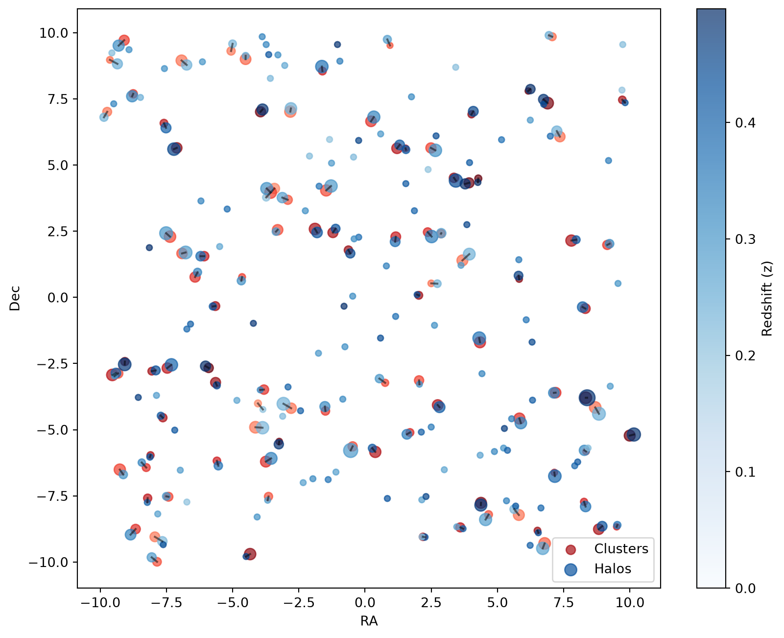
The three strategies trade completeness against uniqueness and confidence. The table below compares them on the filtered 3D matches:
Code
greedy_best = result.select_best(mask=mask)

HTML(
    pd.DataFrame(
        {
            "Strategy": [
                "select_best (greedy)",
                "select_best_assignment",
                "cross match (mutual best)",
            ],
            "Pairs": [
                len(greedy_best.indices),
                len(best_assignment.indices),
                len(cross_match),
            ],
            "Distinct halos": [
                len(set(greedy_best.indices.tolist())),
                len(set(best_assignment.indices.tolist())),
                len(cross_match),
            ],
            "One-to-one": ["not guaranteed", "guaranteed", "guaranteed"],
        }
    ).to_html(index=False)
)| Strategy | Pairs | Distinct halos | One-to-one |
|---|---|---|---|
| select_best (greedy) | 100 | 100 | not guaranteed |
| select_best_assignment | 100 | 100 | guaranteed |
| cross match (mutual best) | 100 | 100 | guaranteed |
For these well-separated mock catalogs the greedy and assignment results coincide, but only the assignment guarantees a one-to-one mapping, which matters whenever candidates contend for the same object. The mutual-best cross match is the most conservative: it keeps the fewest pairs, retaining only those that are reciprocally each other’s best.
When the Methods Disagree
On the well-separated catalog above the three strategies nearly coincide. They diverge when objects contend for the same match — for instance when a cluster finder splits a single halo into several detections. To see this, we build a small catalog in which five of the ten halos are each detected as three clusters (two more halos are detected once, and the last two are missed), plus two spurious detections with no associated halo.
def radecz_to_xyz(ra, dec, z):
    r = np.array(dist.comoving_array(cosmo, np.atleast_1d(z))) * cosmo.RH_Mpc()
    return (
        r * np.cos(np.radians(dec)) * np.cos(np.radians(ra)),
        r * np.cos(np.radians(dec)) * np.sin(np.radians(ra)),
        r * np.sin(np.radians(dec)),
    )


def xyz_to_radecz(x, y, z):
    r = np.sqrt(x * x + y * y + z * z)
    return (
        np.degrees(np.arctan2(y, x)),
        np.degrees(np.arcsin(z / r)),
        np.array([dist.inv_comoving(cosmo, ri / cosmo.RH_Mpc()) for ri in r]),
    )


rng_c = np.random.default_rng(11)

halo_ra_c = rng_c.uniform(RA_MIN, RA_MAX, 10)
halo_dec_c = rng_c.uniform(DEC_MIN, DEC_MAX, 10)
halo_z_c = rng_c.uniform(0.3, 0.4, 10)
hx, hy, hz = radecz_to_xyz(halo_ra_c, halo_dec_c, halo_z_c)

# Halos 0-4 are each detected three times (fragmentation); 5-7 once; 8-9 missed.
parents = np.array([0, 0, 0, 1, 1, 1, 2, 2, 2, 3, 3, 3, 4, 4, 4, 5, 6, 7])
scatter = 25.0
cx = hx[parents] + rng_c.uniform(-scatter, scatter, parents.size)
cy = hy[parents] + rng_c.uniform(-scatter, scatter, parents.size)
cz = hz[parents] + rng_c.uniform(-scatter, scatter, parents.size)
cluster_ra_c, cluster_dec_c, cluster_z_c = xyz_to_radecz(cx, cy, cz)

# Two spurious detections with no underlying halo.
cluster_ra_c = np.append(cluster_ra_c, rng_c.uniform(RA_MIN, RA_MAX, 2))
cluster_dec_c = np.append(cluster_dec_c, rng_c.uniform(DEC_MIN, DEC_MAX, 2))
cluster_z_c = np.append(cluster_z_c, rng_c.uniform(0.3, 0.4, 2))

clusters_c = Table(
    [cluster_ra_c, cluster_dec_c, cluster_z_c], names=["RA", "DEC", "z"]
)
halos_c = Table([halo_ra_c, halo_dec_c, halo_z_c], names=["RA", "DEC", "z"])
coords_c = Coordinates(RA="RA", DEC="DEC", z="z")

sm_c = SkyMatch(clusters_c, coords_c, halos_c, coords_c)
result_c = sm_c.match_3d(cosmo, n_nearest_neighbours=4)
mask_c = result_c.filter_mask_by_distance(60.0)

greedy_c = result_c.select_best(mask=mask_c)
assignment_c = result_c.select_best_assignment(mask=mask_c)

inverse_c = sm_c.invert_query_match()
inverse_result_c = inverse_c.match_3d(cosmo, n_nearest_neighbours=4)
inverse_best_c = inverse_result_c.select_best(
    mask=inverse_result_c.filter_mask_by_distance(60.0)
)
cross_c = greedy_c.get_cross_match_indices(inverse_best_c)
Greedy lets both detections of a fragmented halo keep it, so that halo is matched twice; the assignment forces a one-to-one mapping; the cross match keeps only mutual bests:
Code
HTML(
    pd.DataFrame(
        {
            "Strategy": [
                "select_best (greedy)",
                "select_best_assignment",
                "cross match (mutual best)",
            ],
            "Pairs": [len(greedy_c.indices), len(assignment_c.indices), len(cross_c)],
            "Distinct halos": [
                len(set(greedy_c.indices.tolist())),
                len(set(assignment_c.indices.tolist())),
                len(cross_c),
            ],
        }
    ).to_html(index=False)
)| Strategy | Pairs | Distinct halos |
|---|---|---|
| select_best (greedy) | 18 | 8 |
| select_best_assignment | 9 | 9 |
| cross match (mutual best) | 8 | 8 |
The plot makes the difference concrete: in the greedy panel each of the five fragmented halos sits at the centre of a fan of three clusters (the colliding detections), while the assignment panel keeps a single cluster per halo — and reassigns some of the displaced detections to other nearby halos.
Code
def plot_strategy(ax, candidates, title):
    ax.scatter(halo_ra_c, halo_dec_c, c="red", label="Halos", alpha=0.7)
    ax.scatter(cluster_ra_c, cluster_dec_c, c="blue", label="Clusters", alpha=0.7)
    for cluster_i, halo_i in zip(candidates.query_indices, candidates.indices):
        ax.plot(
            [cluster_ra_c[cluster_i], halo_ra_c[halo_i]],
            [cluster_dec_c[cluster_i], halo_dec_c[halo_i]],
            color="black",
            alpha=0.5,
        )
    ax.set_title(title)
    ax.set_xlabel("RA")
    ax.set_ylabel("Dec")


fig, (ax_greedy, ax_assign) = plt.subplots(
    1, 2, figsize=(14, 6), sharex=True, sharey=True
)
plot_strategy(ax_greedy, greedy_c, "Greedy select_best")
plot_strategy(ax_assign, assignment_c, "select_best_assignment")
ax_greedy.legend()
plt.show()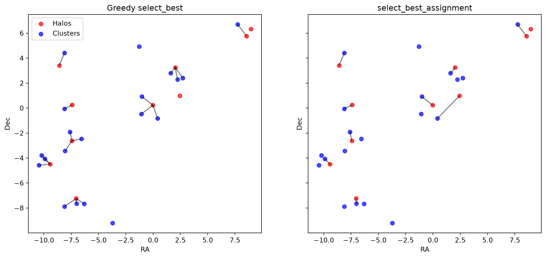
Which behaviour is appropriate depends on the question being asked. If a halo can legitimately host several detections, the many-to-one greedy result is correct and the assignment would discard valid associations. If instead you need a deduplicated, one-to-one catalog cross-match, select_best_assignment gives the globally optimal mapping, and the mutual-best cross match gives the smaller high-confidence subset.
2D Sky Match
The match_2d method functions similarly to match_3d but performs a 2D match instead of a 3D one. In practice, it matches clusters to halos within the same plane of the sky, which is particularly useful when redshift measurement errors are significant.
In a 2D match, the angular separation between clusters and halos is first computed and then converted to a physical distance. This conversion can be performed using different reference redshifts: the cluster redshift, the halo redshift, or the minimum/maximum of the two. The choice is controlled by the distance_method parameter, which accepts the following options:
DistanceMethod.ANGULAR_SEPARATION(computes only the angular separation)
DistanceMethod.QUERY_RADIUS(uses the cluster redshift)
DistanceMethod.MATCH_RADIUS(uses the halo redshift)
DistanceMethod.MIN_RADIUS(uses the minimum redshift)
DistanceMethod.MAX_RADIUS(uses the maximum redshift)
The 2D matching process is performed using the match_2d method. Below is an example of how it works:
# Perform 2D matching
# Keeping the number of nearest neighbors to 6
result = sm.match_2d(
    cosmo, n_nearest_neighbours=6, distance_method=DistanceMethod.QUERY_RADIUS
)
Here, result contains the distances between clusters and halos, computed using the cluster redshifts. The table below shows these distances in mega-parsecs (Mpc):
Code
show_pandas(convert_table_multi_column(result.to_table_complete()).to_pandas())| ID | RA | DEC | z | ID_matched | distances | RA_matched | DEC_matched | z_matched | |
|---|---|---|---|---|---|---|---|---|---|
| 0 | 0 | -5.65 | -0.33 | 0.43 | [ 0 114 44 131 65 170] | [ 1.93 23.4 27.67 27.94 29.18 31.85] | [-5.74 -6.59 -4.67 -6.73 -6.32 -4.21] | [-0.34 -1.01 0.63 -1.2 0.95 -0.98] | [0.43 0.41 0.31 0.39 0.34 0.48] |
| 1 | 1 | 6.51 | -8.81 | 0.44 | [ 1 118 10 133 9 117] | [ 1.8 12.73 14.35 17.69 24.31 25.24] | [6.54 6.23 6.71 6.64 5.63 5.69] | [-8.89 -9.37 -9.48 -7.96 -8. -7.89] | [0.44 0.41 0.27 0.39 0.23 0.42] |
| 2 | 2 | 7.07 | 9.85 | 0.25 | [ 2 18 24 127 134 147] | [ 1.86 29.94 33.46 36.02 36.98 45.58] | [6.95 6.25 6.74 6.75 9.73 6.24] | [9.9 7.87 7.48 7.3 9.55 6.7 ] | [0.25 0.5 0.48 0.44 0.22 0.29] |
| 3 | 3 | 4.02 | 6.92 | 0.45 | [ 3 168 162 119 132 43] | [ 2.75 30.82 32.45 38.02 38.99 39.98] | [4.09 5.15 2.68 3.95 3.42 2.66] | [7.03 5.96 6.1 5.09 8.7 5.56] | [0.45 0.37 0.45 0.42 0.21 0.31] |
| 4 | 4 | 8.27 | -7.72 | 0.36 | [ 4 41 121 78 97 151] | [ 3.43 20.87 25.67 26.7 27.79 27.82] | [8.33 8.95 7.92 7.17 9.53 8.03] | [-7.9 -8.65 -6.36 -6.75 -8.6 -6.22] | [0.37 0.43 0.39 0.39 0.36 0.42] |
| ... | ... | ... | ... | ... | ... | ... | ... | ... | ... |
| 95 | 95 | 7.20 | -3.60 | 0.34 | [ 95 125 86 96 7 156] | [ 1.17 15.98 21.03 30.41 31.74 33.68] | [7.13 6.32 8.39 5.88 8.83 5.54] | [-3.61 -3.88 -3.79 -4.75 -4.4 -4.59] | [0.34 0.41 0.49 0.34 0.25 0.35] |
| 96 | 96 | 5.83 | -4.58 | 0.34 | [ 96 156 195 125 144 169] | [ 3.13 5.14 11.89 14.94 22.19 22.48] | [5.88 5.54 5.26 6.32 5.23 5.38] | [-4.75 -4.59 -4.95 -3.88 -5.69 -5.78] | [0.34 0.35 0.47 0.41 0.3 0.41] |
| 97 | 97 | 9.50 | -8.67 | 0.36 | [ 97 41 4 121 151 10] | [ 1.23 9.84 25.23 50.61 51.73 52.19] | [9.53 8.95 8.33 7.92 8.03 6.71] | [-8.6 -8.65 -7.9 -6.36 -6.22 -9.48] | [0.36 0.43 0.37 0.39 0.42 0.27] |
| 98 | 98 | 8.32 | -0.42 | 0.40 | [ 98 143 146 101 57 53] | [ 2.26 30.23 44.09 46.1 50.76 50.94] | [8.22 9.55 6.09 6.31 9.23 7.97] | [-0.37 0.53 -0.85 -1.69 2.03 2.18] | [0.4 0.31 0.37 0.45 0.32 0.42] |
| 99 | 99 | -4.51 | 9.00 | 0.26 | [ 99 71 160 150 140 145] | [ 1.8 10.88 12.67 13.61 15.13 16.91] | [-4.51 -5. -3.64 -3.73 -3.88 -3.57] | [9.13 9.58 9.17 9.55 9.85 8.28] | [0.26 0.23 0.43 0.33 0.34 0.23] |
Since this method assumes both objects share the same redshift (equal to the cluster redshift), the computed distances are generally smaller than their 3D counterparts. In 3D matching, the full spatial separation is considered, whereas in 2D matching, the calculated distance serves as a lower bound rather than the true three-dimensional separation. See Table 3 for comparison.
If we had used halo redshifts instead, we would still obtain a lower bound on the distance, but this time computed assuming the halos’ redshifts rather than the clusters’.
Filtering Results
To refine the matching process, we apply filters based on distance and redshift criteria.
Since the computed distances provide only a lower bound—meaning the actual 3D separations could be larger, we set a distance threshold of 60 Mpc to exclude pairs that are likely too far apart.
Additionally, we apply a redshift filter, retaining only pairs where the redshift difference is below 0.02, ensuring the matches remain within a physically relevant range.
# Apply a distance filter to retain only matches within 60 Mpc
mask = result.filter_mask_by_distance(60.0)

# Further refine by keeping only matches with redshift < 0.02
mask = result.filter_mask_by_redshift_proximity(0.02, mask=mask)
These filters help isolate the most relevant cluster-halo associations for further analysis.
The filtered table is shown below:
Code
show_pandas(convert_table_multi_column(result.to_table_complete(mask)).to_pandas())| ID | RA | DEC | z | ID_matched | distances | RA_matched | DEC_matched | z_matched | |
|---|---|---|---|---|---|---|---|---|---|
| 0 | 0 | -5.65 | -0.33 | 0.43 | [ 0 114 131 170] | [ 1.93 23.4 27.94 31.85] | [-5.74 -6.59 -6.73 -4.21] | [-0.34 -1.01 -1.2 -0.98] | [0.43 0.41 0.39 0.48] |
| 1 | 1 | 6.51 | -8.81 | 0.44 | [ 1 118 133 117] | [ 1.8 12.73 17.69 25.24] | [6.54 6.23 6.64 5.69] | [-8.89 -9.37 -7.96 -7.89] | [0.44 0.41 0.39 0.42] |
| 2 | 2 | 7.07 | 9.85 | 0.25 | [ 2 134 147] | [ 1.86 36.98 45.58] | [6.95 9.73 6.24] | [9.9 9.55 6.7 ] | [0.25 0.22 0.29] |
| 3 | 3 | 4.02 | 6.92 | 0.45 | [ 3 162 119] | [ 2.75 32.45 38.02] | [4.09 2.68 3.95] | [7.03 6.1 5.09] | [0.45 0.45 0.42] |
| 4 | 4 | 8.27 | -7.72 | 0.36 | [ 4 121 78 97 151] | [ 3.43 25.67 26.7 27.79 27.82] | [8.33 7.92 7.17 9.53 8.03] | [-7.9 -6.36 -6.75 -8.6 -6.22] | [0.37 0.39 0.39 0.36 0.42] |
| ... | ... | ... | ... | ... | ... | ... | ... | ... | ... |
| 95 | 95 | 7.20 | -3.60 | 0.34 | [ 95 96 156] | [ 1.17 30.41 33.68] | [7.13 5.88 5.54] | [-3.61 -4.75 -4.59] | [0.34 0.34 0.35] |
| 96 | 96 | 5.83 | -4.58 | 0.34 | [ 96 156 144] | [ 3.13 5.14 22.19] | [5.88 5.54 5.23] | [-4.75 -4.59 -5.69] | [0.34 0.35 0.3 ] |
| 97 | 97 | 9.50 | -8.67 | 0.36 | [ 97 4 121] | [ 1.23 25.23 50.61] | [9.53 8.33 7.92] | [-8.6 -7.9 -6.36] | [0.36 0.37 0.39] |
| 98 | 98 | 8.32 | -0.42 | 0.40 | [ 98 146 101 53] | [ 2.26 44.09 46.1 50.94] | [8.22 6.09 6.31 7.97] | [-0.37 -0.85 -1.69 2.18] | [0.4 0.37 0.45 0.42] |
| 99 | 99 | -4.51 | 9.00 | 0.26 | [ 99 71 145] | [ 1.8 10.88 16.91] | [-4.51 -5. -3.57] | [9.13 9.58 8.28] | [0.26 0.23 0.23] |
The plot below illustrates the filtered results:
Code
plot_mask(mask)
plt.show()
The refined selection highlights cluster-halo pairs that are both spatially and redshift-wise well-matched within the relevant observational range.
Best Match Selection
To further refine the associations, we use the select_best method to identify the most suitable halo for each cluster.
We specify the selection_criteria as MORE_MASSIVE, meaning we select the halo with the largest halo_logM value as the best match.
# Find the best match for each cluster
best = result.select_best(
    selection_criteria=SelectionCriteria.MORE_MASSIVE,
    mask=mask,
    more_massive_column="halo_logM",
)
This results in a BestCandidates object containing the indices of the most likely halo match for each cluster. The table below presents the selected best matches, along with the corresponding cluster and halo masses:
Code
show_pandas(
    convert_table_multi_column(
        result.to_table_best(
            best,
            query_properties={"cluster_logM": "cluster_logM"},
            match_properties={"halo_logM": "halo_logM"},
        )
    ).to_pandas()
)| ID | RA | DEC | z | ID_matched | RA_matched | DEC_matched | z_matched | cluster_logM | halo_logM | |
|---|---|---|---|---|---|---|---|---|---|---|
| 0 | 0 | -5.65 | -0.33 | 0.43 | 0 | -5.74 | -0.34 | 0.43 | 13.83 | 13.32 |
| 1 | 1 | 6.51 | -8.81 | 0.44 | 118 | 6.23 | -9.37 | 0.41 | 13.20 | 12.56 |
| 2 | 2 | 7.07 | 9.85 | 0.25 | 2 | 6.95 | 9.9 | 0.25 | 13.55 | 13.46 |
| 3 | 3 | 4.02 | 6.92 | 0.45 | 3 | 4.09 | 7.03 | 0.45 | 13.32 | 14.19 |
| 4 | 4 | 8.27 | -7.72 | 0.36 | 78 | 7.17 | -6.75 | 0.39 | 13.32 | 15.36 |
| ... | ... | ... | ... | ... | ... | ... | ... | ... | ... | ... |
| 95 | 95 | 7.20 | -3.60 | 0.34 | 96 | 5.88 | -4.75 | 0.34 | 14.49 | 14.90 |
| 96 | 96 | 5.83 | -4.58 | 0.34 | 96 | 5.88 | -4.75 | 0.34 | 14.68 | 14.90 |
| 97 | 97 | 9.50 | -8.67 | 0.36 | 4 | 8.33 | -7.9 | 0.37 | 13.13 | 14.40 |
| 98 | 98 | 8.32 | -0.42 | 0.40 | 98 | 8.22 | -0.37 | 0.4 | 14.17 | 14.42 |
| 99 | 99 | -4.51 | 9.00 | 0.26 | 71 | -5. | 9.58 | 0.23 | 14.53 | 13.48 |
The plot below visualizes the best matches:
Code
plot_best(best)
plt.show()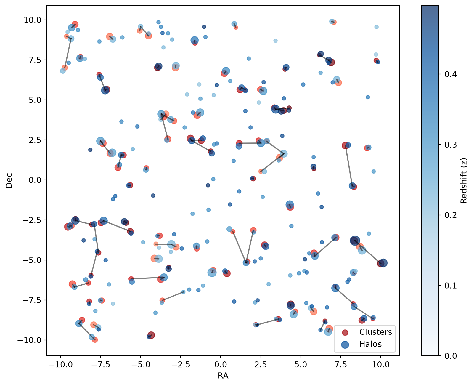
This final selection ensures that each cluster is associated with the most massive halo within the given constraints, optimizing the matching process.
Best Match by Global Assignment
Just as in 3D, select_best_assignment provides a one-to-one alternative to the greedy select_best. It is especially relevant in 2D, where the larger positional and redshift uncertainties make it more likely that several clusters would otherwise claim the same halo. It accepts the same filtered mask and returns the familiar BestCandidates:
best_assignment = result.select_best_assignment(mask=mask)Code
plot_best(best_assignment)
plt.show()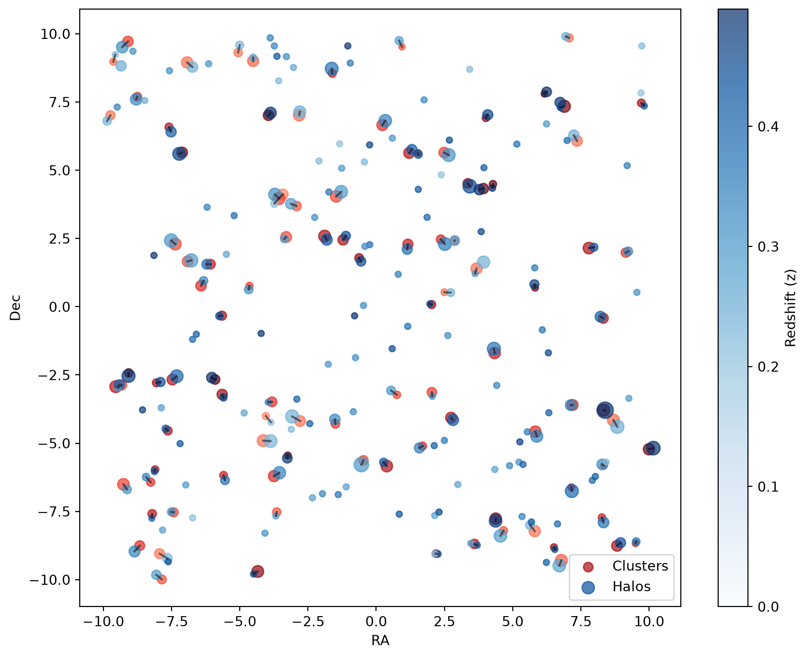
Cross Matching
To improve the accuracy of our cluster-halo associations, we invert the catalogs with invert_query_match and combine the two best-match results with get_cross_match_indices to identify the best match for each halo. Previously, in Table 11, we selected the best match for each cluster. However, since we did not use actual distances, some incorrect matches may have been included.
By applying cross_match from the halo perspective, we refine the matching process.
# Find the best match for each halo

cross = sm.invert_query_match()

cross_result = cross.match_2d(cosmo, n_nearest_neighbours=6)

cross_mask = cross_result.filter_mask_by_distance(60.0)
cross_mask = cross_result.filter_mask_by_redshift_proximity(0.02, mask=cross_mask)

cross_best = cross_result.select_best(
    selection_criteria=SelectionCriteria.REDSHIFT_PROXIMITY, mask=cross_mask
)

cross_match = best.get_cross_match_indices(cross_best)
This results in a BestCandidates object containing the indices of the most probable cluster match for each halo.
The table below presents the selected best matches along with the corresponding cluster and halo masses:
Code
show_pandas(
    convert_table_multi_column(
        cross_result.to_table_best(
            cross_best,
            query_properties={"halo_logM": "halo_logM"},
            match_properties={"cluster_logM": "cluster_logM"},
        )
    ).to_pandas()
)| ID | RA | DEC | z | ID_matched | RA_matched | DEC_matched | z_matched | halo_logM | cluster_logM | |
|---|---|---|---|---|---|---|---|---|---|---|
| 0 | 0 | -5.74 | -0.34 | 0.43 | 0 | -5.65 | -0.33 | 0.43 | 13.32 | 13.83 |
| 1 | 1 | 6.54 | -8.89 | 0.44 | 1 | 6.51 | -8.81 | 0.44 | 12.52 | 13.20 |
| 2 | 2 | 6.95 | 9.90 | 0.25 | 2 | 7.07 | 9.85 | 0.25 | 13.46 | 13.55 |
| 3 | 3 | 4.09 | 7.03 | 0.45 | 3 | 4.02 | 6.92 | 0.45 | 14.19 | 13.32 |
| 4 | 4 | 8.33 | -7.90 | 0.37 | 4 | 8.27 | -7.72 | 0.36 | 14.40 | 13.32 |
| ... | ... | ... | ... | ... | ... | ... | ... | ... | ... | ... |
| 184 | 194 | -9.49 | 7.31 | 0.34 | 67 | -8.75 | 7.69 | 0.33 | 12.92 | 13.70 |
| 185 | 196 | -6.97 | -6.53 | 0.29 | 19 | -7.42 | -7.53 | 0.3 | 10.08 | 13.85 |
| 186 | 197 | 9.19 | 5.17 | 0.35 | 57 | 9.15 | 1.98 | 0.32 | 12.28 | 13.95 |
| 187 | 198 | 3.62 | 1.21 | 0.29 | 80 | 2.87 | 2.41 | 0.28 | 10.13 | 13.65 |
| 188 | 199 | 8.42 | -5.69 | 0.22 | 7 | 8.69 | -4.16 | 0.25 | 10.91 | 14.92 |
The following plot visualizes the cross matches:
Code
plot_cross(cross_match)
plt.show()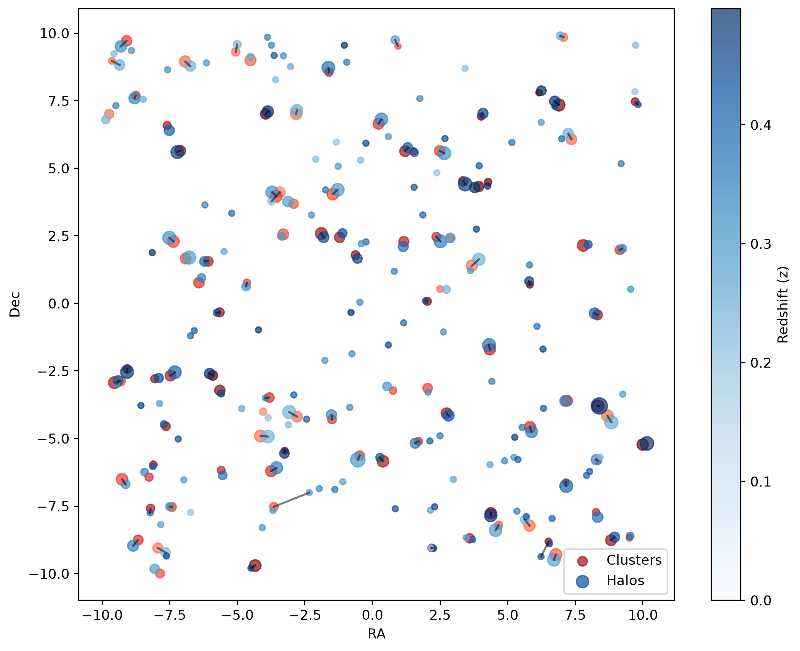
In the final step, we assess the best match for each cluster by inspecting the cross_match dictionary, which stores the indices of the best matches.
We then evaluate the total number of matches, as well as the proportion of correct and incorrect assignments.
Code
# Convert dictionary to DataFrame for better visualization
cross_match_df = pd.DataFrame(
    list(cross_match.items()), columns=["Cluster ID", "Matched Halo ID"]
)

# Compute correctness
wrong = cross_match_df["Cluster ID"] != cross_match_df["Matched Halo ID"]
right = ~wrong  # Logical NOT for correct matches

# Add correctness column
cross_match_df["Correct Match"] = right

cross_match_df| Cluster ID | Matched Halo ID | Correct Match | |
|---|---|---|---|
| 0 | 0 | 0 | True |
| 1 | 1 | 118 | False |
| 2 | 2 | 2 | True |
| 3 | 3 | 3 | True |
| 4 | 5 | 5 | True |
| ... | ... | ... | ... |
| 63 | 90 | 90 | True |
| 64 | 92 | 92 | True |
| 65 | 94 | 94 | True |
| 66 | 96 | 96 | True |
| 67 | 98 | 98 | True |
68 rows × 3 columns
The match statistics are summarized below:
Code
# Display match statistics
HTML(
    pd.DataFrame(
        {
            "Total Matches": [len(cross_match)],
            "Correct Matches": [right.sum()],
            "Wrong Matches": [wrong.sum()],
        }
    ).to_html(index=False)
)| Total Matches | Correct Matches | Wrong Matches |
|---|---|---|
| 68 | 66 | 2 |
In summary, we have successfully matched the clusters with the halos, keeping in mind that the artificial dataset was intentionally generated with increased errors to enhance visibility. As a result, some incorrect or suboptimal matches were expected.
Finally, we compare the three selection strategies on these 2D matches. Because cluster i was generated near halo i, a match is correct when the assigned halo index equals the cluster index:
Code
greedy_2d = result.select_best(mask=mask)
assignment_2d = result.select_best_assignment(mask=mask)


def count_correct(candidates):
    return sum(
        1
        for q, m in zip(candidates.query_indices, candidates.indices)
        if q == m
    )


HTML(
    pd.DataFrame(
        {
            "Strategy": [
                "select_best (greedy)",
                "select_best_assignment",
                "cross match (mutual best)",
            ],
            "Pairs": [
                len(greedy_2d.indices),
                len(assignment_2d.indices),
                len(cross_match),
            ],
            "Correct": [
                count_correct(greedy_2d),
                count_correct(assignment_2d),
                sum(1 for q, m in cross_match.items() if q == m),
            ],
        }
    ).to_html(index=False)
)| Strategy | Pairs | Correct |
|---|---|---|
| select_best (greedy) | 100 | 97 |
| select_best_assignment | 100 | 97 |
| cross match (mutual best) | 68 | 66 |
Here the greedy and assignment strategies keep every cluster with the same number of correct matches, but only the assignment guarantees that no halo is reused. The mutual-best cross match keeps far fewer pairs: it is the conservative choice, paying in completeness for its reciprocity requirement, which is most worthwhile when the matches are genuinely ambiguous (as in the contended example above).
Summary
This tutorial demonstrated NumCosmo’s SkyMatch class as a robust tool for cross-matching galaxy clusters with simulated dark matter halos. Using mock datasets, 100 clusters and 200 halos (100 spatially correlated with clusters, 100 randomly distributed), we showcased two key methodologies:
- match_3d: Achieves precise associations using 3D positional and redshift data, ideal for spectroscopic surveys.
- match_2d: Relies on angular proximity, critical for photometric surveys or datasets with redshift uncertainties.
Cross-validation via cross_match and statistical analysis revealed that correlated halos (positioned near clusters) were reliably matched, while mismatches arose primarily from random halos or positional noise. This underscores the importance of probabilistic matching (match_2d) and systematic validation in real-world scenarios, where overlapping structures and observational errors are common.
By quantifying completeness (successful cluster-halo matches) and purity (minimizing false associations), the SkyMatch framework enables rigorous evaluation of observational catalogs. While simplified mock data omitted complexities like mass-observable scatter or projection effects, the workflow mirrors steps essential for cosmological analyses, such as calibrating selection functions for cluster abundance studies.
Tools like SkyMatch bridge simulations and observations, allowing to diagnose catalog reliability and refine strategies for upcoming surveys (e.g., LSST, Euclid), where accurate matching will be crucial for constraining dark energy and structure growth.