Matching by Shared Membership

def doc_theme():
    return theme_minimal() + theme(
        panel_grid_minor=element_line(color="gray", linetype="--"),
    )

Purpose

The companion tutorial Matching Observations to Simulations matches objects by their positions on the sky. NumCosmo’s sky_match module also supports a complementary strategy: matching objects by their shared members.

Many catalogs describe extended objects (galaxy clusters, halos) as collections of member galaxies. When two catalogs are built from the same underlying galaxies, two objects can be associated by how many members they have in common, regardless of their catalog positions. This is what the match_ID method does: it links a query object to a match object whenever they share member galaxies, and scores each candidate link with a linking coefficient.

In this tutorial we build a pair of mock catalogs of halos and detected clusters, each described by a member catalog, and use match_ID to associate them.

Member Catalogs

Membership matching needs two pieces of information per catalog:

• an object catalog, with one row per object and a unique object ID, and
• a member catalog, with one row per member, mapping each member (e.g. a galaxy) to the object it belongs to and, optionally, a probability of membership pmem.

We generate 35 matched halo/cluster pairs plus a handful of unmatched field objects in each catalog. Each object has 10 members; a matched halo and its cluster share 7 of them, so the expected Jaccard overlap is \(7 / (10 + 10 - 7) \approx 0.54\). Member galaxies carry a random pmem to illustrate the probability-weighted methods later on. Object positions are generated too — matched pairs sit close together — but note that positions are not used by match_ID; they only help visualize the result.

import numpy as np
import pandas as pd
from astropy.table import Table
from IPython.display import HTML

from numcosmo_py import Ncm
from numcosmo_py.catalog import (
    SkyMatch,
    Coordinates,
    IDs,
    SharedFractionMethod,
)

Ncm.cfg_init()
rng = np.random.default_rng(123)

N_MATCHED, N_FIELD = 35, 5
N_MEM, N_SHARED = 10, 7
RA_MIN, RA_MAX = -10.0, 10.0
DEC_MIN, DEC_MAX = -10.0, 10.0
Z_MIN, Z_MAX = 0.2, 0.5


def random_position():
    return (
        rng.uniform(RA_MIN, RA_MAX),
        rng.uniform(DEC_MIN, DEC_MAX),
        rng.uniform(Z_MIN, Z_MAX),
    )


galaxy_id = 0
halo_members, cluster_members = [], []
halo_objects, cluster_objects = [], []

# Matched pairs: the cluster shares N_SHARED of the halo's galaxies.
for i in range(N_MATCHED):
    halo_gals = list(range(galaxy_id, galaxy_id + N_MEM))
    galaxy_id += N_MEM
    shared = halo_gals[:N_SHARED]
    new_gals = list(range(galaxy_id, galaxy_id + (N_MEM - N_SHARED)))
    galaxy_id += N_MEM - N_SHARED
    cluster_gals = shared + new_gals

    for g in halo_gals:
        halo_members.append((i, g, rng.uniform(0.6, 1.0)))
    for g in cluster_gals:
        cluster_members.append((1000 + i, g, rng.uniform(0.6, 1.0)))

    ra, dec, z = random_position()
    halo_objects.append((i, ra, dec, z))
    cluster_objects.append((1000 + i, ra + rng.normal(0, 0.2), dec + rng.normal(0, 0.2), z))

# Field objects: members that are not shared with the other catalog.
for i in range(N_FIELD):
    for g in range(galaxy_id, galaxy_id + N_MEM):
        halo_members.append((500 + i, g, rng.uniform(0.6, 1.0)))
    galaxy_id += N_MEM
    halo_objects.append((500 + i, *random_position()))
for i in range(N_FIELD):
    for g in range(galaxy_id, galaxy_id + N_MEM):
        cluster_members.append((2000 + i, g, rng.uniform(0.6, 1.0)))
    galaxy_id += N_MEM
    cluster_objects.append((2000 + i, *random_position()))

halo_data = Table(rows=halo_objects, names=["halo_id", "RA", "DEC", "z"])
cluster_data = Table(rows=cluster_objects, names=["cluster_id", "RA", "DEC", "z"])
halo_member_data = Table(rows=halo_members, names=["halo_id", "galaxy_id", "pmem"])
cluster_member_data = Table(rows=cluster_members, names=["cluster_id", "galaxy_id", "pmem"])

The object and member catalogs for the halos look like this (clusters are analogous):

def show_pandas(df: pd.DataFrame):
    return HTML(df.to_html(float_format="%.2f", max_rows=10))


show_pandas(halo_data.to_pandas())

	halo_id	RA	DEC	z
0	0	-5.37	-6.68	0.35
1	1	-3.75	-9.71	0.21
2	2	-0.29	0.38	0.32
3	3	-1.51	-6.97	0.46
4	4	9.21	0.87	0.40
...	...	...	...	...
35	500	4.20	8.22	0.25
36	501	-0.34	2.94	0.48
37	502	-2.24	-0.78	0.40
38	503	-4.79	9.37	0.31
39	504	2.98	-4.98	0.22

Table 1: The halo object catalog (left) and the first rows of its member catalog (right).

show_pandas(halo_member_data.to_pandas())

	halo_id	galaxy_id	pmem
0	0	0	0.87
1	0	1	0.62
2	0	2	0.69
3	0	3	0.67
4	0	4	0.67
...	...	...	...
395	504	500	0.85
396	504	501	0.86
397	504	502	0.92
398	504	503	0.92
399	504	504	0.98

Table 2: The first rows of the halo member catalog.

Building the SkyMatch

The SkyMatch object now receives, in addition to the object catalogs and their Coordinates, the member catalogs and an IDs map that names the object-ID, member-ID, and (optional) pmem columns in each member catalog.

halo_coords = Coordinates(RA="RA", DEC="DEC", z="z")
cluster_coords = Coordinates(RA="RA", DEC="DEC", z="z")

halo_ids = IDs(ID="halo_id", MemberID="galaxy_id", pmem="pmem")
cluster_ids = IDs(ID="cluster_id", MemberID="galaxy_id", pmem="pmem")

sm = SkyMatch(
    query_data=halo_data,
    query_coordinates=halo_coords,
    query_member_data=halo_member_data,
    query_ids=halo_ids,
    match_data=cluster_data,
    match_coordinates=cluster_coords,
    match_member_data=cluster_member_data,
    match_ids=cluster_ids,
)

Membership Matching

The match_ID method joins the two member catalogs on the shared member IDs and groups the result by query/match object pairs. By default the linking coefficient is the Jaccard index of the two member sets,

\[ J = \frac{|M_\text{query} \cap M_\text{match}|}{|M_\text{query} \cup M_\text{match}|}, \]

so for our matched pairs \(J = 7 / 13 \approx 0.54\).

result = sm.match_ID()

The result is a SkyMatchIDResult. Unlike the distance-based SkyMatchResult, the candidate lists are ragged: each query object may share members with any number of match objects (or none). The to_table_complete method lays out every candidate per query, with its linking coefficient:

def stringify_candidate_columns(table):
    for col in ["match_id", "linking_coefficient", "RA_matched", "DEC_matched", "z_matched"]:
        table[col] = [np.array2string(np.asarray(v), precision=2) for v in table[col]]
    return table


show_pandas(stringify_candidate_columns(result.to_table_complete()).to_pandas())

	query_id	RA	DEC	z	match_id	linking_coefficient	RA_matched	DEC_matched	z_matched
0	0	-5.37	-6.68	0.35	[1000]	[0.54]	[-5.14]	[-6.53]	[0.35]
1	1	-3.75	-9.71	0.21	[1001]	[0.54]	[-3.29]	[-9.85]	[0.21]
2	2	-0.29	0.38	0.32	[1002]	[0.54]	[-0.33]	[0.46]	[0.32]
3	3	-1.51	-6.97	0.46	[1003]	[0.54]	[-1.76]	[-7.03]	[0.46]
4	4	9.21	0.87	0.40	[1004]	[0.54]	[9.37]	[0.8]	[0.4]
...	...	...	...	...	...	...	...	...	...
35	500	4.20	8.22	0.25	[]	[]	[]	[]	[]
36	501	-0.34	2.94	0.48	[]	[]	[]	[]	[]
37	502	-2.24	-0.78	0.40	[]	[]	[]	[]	[]
38	503	-4.79	9.37	0.31	[]	[]	[]	[]	[]
39	504	2.98	-4.98	0.22	[]	[]	[]	[]	[]

Table 3: All candidate matches per halo with their linking (Jaccard) coefficients.

The field halos (IDs 500–504) share no members with any cluster, so their candidate lists are empty.

Best Match

select_best resolves a one-to-one matching. It builds the bipartite graph of candidate links (weighted by the linking coefficient), splits it into connected components, and runs a maximum-weight matching on each, so no cluster is assigned to more than one halo and the total linking coefficient is maximized.

best = result.select_best()

The returned BestCandidates behaves exactly as in the distance tutorial, and to_table_best produces one row per matched halo:

show_pandas(result.to_table_best(best).to_pandas())

	query_id	RA	DEC	z	match_id	linking_coefficient	RA_matched	DEC_matched	z_matched
0	0	-5.37	-6.68	0.35	1000	0.54	-5.14	-6.53	0.35
1	1	-3.75	-9.71	0.21	1001	0.54	-3.29	-9.85	0.21
2	2	-0.29	0.38	0.32	1002	0.54	-0.33	0.46	0.32
3	3	-1.51	-6.97	0.46	1003	0.54	-1.76	-7.03	0.46
4	4	9.21	0.87	0.40	1004	0.54	9.37	0.80	0.40
...	...	...	...	...	...	...	...	...	...
30	30	-7.11	2.60	0.44	1030	0.54	-7.10	2.74	0.44
31	31	2.48	2.12	0.40	1031	0.54	2.30	1.68	0.40
32	32	4.59	-5.13	0.28	1032	0.54	4.47	-4.96	0.28
33	33	2.73	0.51	0.28	1033	0.54	2.77	0.30	0.28
34	34	0.04	-6.38	0.45	1034	0.54	0.55	-6.35	0.45

Table 4: The best (one-to-one) membership matches.

Only the 35 matched pairs survive; the 5 field halos and 5 field clusters are left unmatched. Although match_ID never looked at the positions, plotting the matched pairs shows that they are indeed spatially coincident:

import matplotlib.pyplot as plt

fig, ax = plt.subplots(figsize=(10, 8))
ax.scatter(halo_data["RA"], halo_data["DEC"], c="red", label="Halos", alpha=0.7)
ax.scatter(cluster_data["RA"], cluster_data["DEC"], c="blue", label="Clusters", alpha=0.7)

for halo_i, cluster_i in zip(best.query_indices, best.indices):
    ax.plot(
        [halo_data["RA"][halo_i], cluster_data["RA"][cluster_i]],
        [halo_data["DEC"][halo_i], cluster_data["DEC"][cluster_i]],
        color="black",
        alpha=0.5,
    )

ax.set_xlabel("Right Ascension (RA) [°]")
ax.set_ylabel("Declination (Dec) [°]")
ax.legend()
plt.show()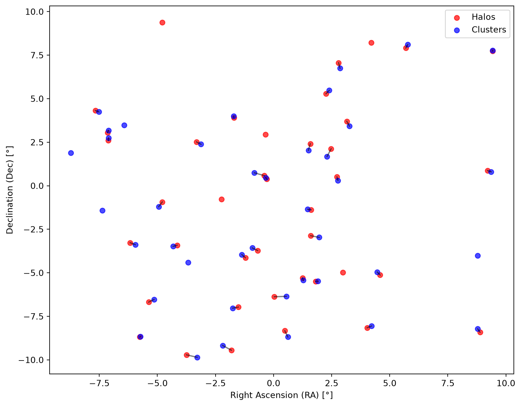

Figure 1: Halos (red) and clusters (blue); black lines connect membership-matched pairs.

Probability-Weighted Membership

The Jaccard index counts members equally. When a probability of membership pmem is available, match_ID(use_shared_fraction=True, ...) weights the shared and total members by their pmem. The shared_fraction_method controls how the shared fraction is formed:

• NO_PMEM: shared member counts (no weighting);
• QUERY_PMEM: weight the shared fraction by the query object’s pmem;
• MATCH_PMEM: weight by the match object’s pmem;
• PMEM: weight by both.

The table below contrasts the linking coefficient of a single matched pair under each method:

rows = []
for method in SharedFractionMethod:
    weighted = method != SharedFractionMethod.NO_PMEM
    method_result = sm.match_ID(use_shared_fraction=weighted, shared_fraction_method=method)
    coeff = float(method_result.candidate_coefficients[0][0])
    rows.append({"method": str(method), "linking coefficient (halo 0)": coeff})

HTML(pd.DataFrame(rows).to_html(index=False, float_format="%.4f"))

method	linking coefficient (halo 0)
no_pmem	0.5385
match_pmem	0.4924
query_pmem	0.4654
pmem	0.4678

Table 5: Linking coefficient of one matched pair under each shared-fraction method.

The exact value depends on the random pmem weights, but all methods agree on the same best matches here, since the membership overlap is unambiguous.

Summary

This tutorial demonstrated NumCosmo’s match_ID, which associates objects by their shared members rather than their positions. We built halo and cluster catalogs with member galaxies, scored candidate links with the Jaccard index (and its probability-weighted variants), and resolved a one-to-one matching with select_best.

Membership matching is the natural choice when both catalogs are built from a common set of tracer galaxies — for example, comparing a cluster finder’s detections to the true halos in a simulation. Combined with the position-based distance matching, the sky_match module covers both regimes with a common result and table interface.