def doc_theme():
    return theme_minimal() + theme(
        panel_grid_minor=element_line(color="gray", linetype="--"),
)Bianchi I Orientation
This page describes the orientation parameters of NcHCosmoBI, the Bianchi I model with pressureless matter and a cosmological constant. The model has three expansion rates today, one per principal axis, and the direction of each observed source enters the distance through its components along those axes. The three parameters \(u_1\), \(u_2\), \(u_3\) fix the rotation from the equatorial frame of the catalog to the frame of the axes. The page states the parametrization, shows that a uniform distribution on the three parameters is the uniform distribution on rotations, and relates the parameters to the hyperspherical angles of the same quaternion.
The model and its frame
The metric is \[
\mathrm{d}s^2 = -\mathrm{d}t^2 + \sum_{i=1}^{3} a_i^2(t)\,\mathrm{d}x_i^2,
\qquad
a_i(t_0) = 1,
\] with the expansion rates \(H_i = \dot a_i / a_i\) along the three axes. The parameters of NcHCosmoBI are \(H_1\), \(H_2\), \(H_3\) today, the matter density parameter \(\Omega_{m0}\), and \(u_1\), \(u_2\), \(u_3\). A source observed from the unit direction \(\hat p\), with equatorial components \((p_x, p_y, p_z)\), has components \(n_i\) along the axes, and its redshift and distance depend on the direction only through \(n_1^2\), \(n_2^2\), \(n_3^2\). The map \(\hat p \mapsto \hat n\) is a rotation.
The rotation as a unit quaternion
A unit quaternion \(q = (s; \vec v)\), with \(s^2 + |\vec v|^2 = 1\), rotates a vector by \[
\hat n = q\,\hat p\,q^\dagger,
\] where \(\hat p\) is the pure quaternion \((0; \hat p)\) and \(q^\dagger = (s; -\vec v)\). This is ncm_quaternion_rotate. The quaternions \(q\) and \(-q\) give the same rotation: the unit quaternions form the sphere \(S^3\), and the rotation group \(SO(3)\) is \(S^3\) with antipodal points identified.
The parameters
The orientation parameters are three numbers in \([0, 1]\), and the quaternion is \[
q(u_1, u_2, u_3) = \Big(\sqrt{u_1}\cos 2\pi u_3;\;
\sqrt{1 - u_1}\,\sin 2\pi u_2,\;
\sqrt{1 - u_1}\,\cos 2\pi u_2,\;
\sqrt{u_1}\,\sin 2\pi u_3\Big),
\] returned by nc_hcosmo_bi_get_quaternion. It is a unit quaternion for every point of the box, since \(u_1 + (1 - u_1) = 1\), and the defaults \((u_1, u_2, u_3) = (1, 0, 0)\) give \(q = (1; 0, 0, 0)\), the identity. Writing \(q = (a; b, c, d)\), the inverse map is \[
u_1 = a^2 + d^2,
\qquad
2\pi u_2 = \arg(c + ib),
\qquad
2\pi u_3 = \arg(a + id),
\] with the arguments taken in \([0, 2\pi)\); this is nc_hcosmo_bi_set_quaternion. The two quaternions \(q\) and \(-q\) map to different points of the box, \((u_1, u_2 + \tfrac12, u_3 + \tfrac12)\) modulo 1, with the same rotation.
Uniform sampling
The uniform distribution on the box \([0, 1]^3\) is the uniform (Haar) distribution on rotations. The uniform distribution on \(SO(3)\) is the uniform distribution on \(S^3\) followed by the identification of \(q\) with \(-q\), so the statement holds if the volume element of \(S^3\) is constant in the coordinates \((u_1, u_2, u_3)\).
Group the four components into two complex numbers, \[ z_1 = a + id = \sqrt{u_1}\,e^{2\pi i u_3}, \qquad z_2 = c + ib = \sqrt{1 - u_1}\,e^{2\pi i u_2}, \] so that \(|z_1|^2 + |z_2|^2 = 1\) and the line element of \(S^3\), inherited from \(\mathbb{R}^4\), is \(\mathrm{d}s^2 = |\mathrm{d}z_1|^2 + |\mathrm{d}z_2|^2\). From \[ \mathrm{d}z_1 = \Big(\frac{\mathrm{d}u_1}{2\sqrt{u_1}} + 2\pi i\sqrt{u_1}\,\mathrm{d}u_3\Big) e^{2\pi i u_3}, \qquad \mathrm{d}z_2 = \Big(-\frac{\mathrm{d}u_1}{2\sqrt{1 - u_1}} + 2\pi i\sqrt{1 - u_1}\,\mathrm{d}u_2\Big) e^{2\pi i u_2}, \] the line element is diagonal, \[ \mathrm{d}s^2 = \frac{\mathrm{d}u_1^2}{4 u_1 (1 - u_1)} + 4\pi^2 (1 - u_1)\,\mathrm{d}u_2^2 + 4\pi^2 u_1\,\mathrm{d}u_3^2, \] and the volume element is the square root of the product of the three coefficients, \[ \mathrm{d}V = \sqrt{\frac{16\pi^4 u_1 (1 - u_1)}{4 u_1 (1 - u_1)}}\;\mathrm{d}u_1\,\mathrm{d}u_2\,\mathrm{d}u_3 = 2\pi^2\,\mathrm{d}u_1\,\mathrm{d}u_2\,\mathrm{d}u_3 . \] The factor is constant and equals the volume of \(S^3\), which the unit box covers once. A sampler that draws \(u_1\), \(u_2\), \(u_3\) uniformly on \([0, 1]\), or with a flat prior on the box, draws rotations uniformly, with no Jacobian.
The chunk below draws \(2 \times 10^6\) points uniformly on the box, checks the constant numerically from the quaternion the model returns, and checks the consequence on the sky: each axis is then uniformly distributed on the sphere, so the component of an axis along any fixed direction is uniform on \([-1, 1]\).
Code
import math
import numpy as np
import matplotlib.pyplot as plt
from numcosmo_py import Nc, Ncm

Ncm.cfg_init()
cosmo = Nc.HCosmoBI.new()


def set_u(u):
    for i, x in enumerate(u):
        cosmo.orig_param_set(Nc.HCosmoBISParams.U1 + i, x)


def quaternion(u):
    set_u(u)
    q = cosmo.get_quaternion()
    return np.array([q.s, q.v.c[0], q.v.c[1], q.v.c[2]])


# The volume element sqrt(det J^T J) of the map box -> S^3 at random points.
rng = np.random.default_rng(1)
h = 1.0e-6
elements = []
for _ in range(5):
    u = rng.uniform(0.05, 0.95, 3)
    J = np.column_stack([(quaternion(u + h * e) - quaternion(u - h * e)) / (2 * h) for e in np.eye(3)])
    elements.append(math.sqrt(np.linalg.det(J.T @ J)))
print("volume element at five random points:", np.round(elements, 6), "; 2 pi^2 =", round(2 * math.pi**2, 6))

# Uniform draws on the box; the angles and axis 3 of each from the model.
n = 2000000
u_draws = rng.uniform(size=(n, 3))
angles = np.empty((n, 3))
z_axis3 = np.empty(n)
for k in range(n):
    set_u(u_draws[k])
    angles[k] = cosmo.get_angles()
    v = Ncm.TriVec.new_full([0.0, 0.0, 1.0])
    cosmo.get_quaternion().rotate(v)
    z_axis3[k] = v.c[2]

fig, axes = plt.subplots(1, 4, figsize=(12, 3))
for i, ax in enumerate(axes[:3]):
    ax.hist(u_draws[:, i], bins=50, range=(0, 1), density=True, histtype="step")
    ax.axhline(1.0, color="C3", lw=1)
    ax.set_xlabel(f"$u_{i + 1}$")
    ax.set_ylim(0, 1.3)
axes[3].hist(z_axis3, bins=50, range=(-1, 1), density=True, histtype="step")
axes[3].axhline(0.5, color="C3", lw=1)
axes[3].set_xlabel("axis 3, component along $z$")
axes[3].set_ylim(0, 0.65)
axes[0].set_ylabel("density")
plt.tight_layout()
plt.show()
volume element at five random points: [19.739209 19.739209 19.739209 19.739209 19.739209] ; 2 pi^2 = 19.739209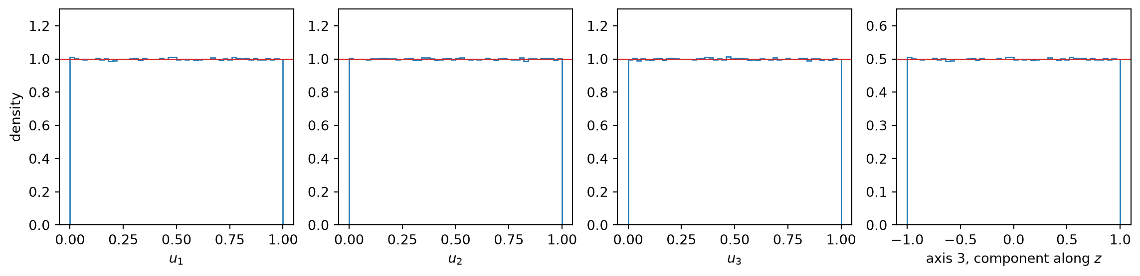
The hyperspherical angles
The same unit quaternion can be written with the spherical coordinates of \(S^3\), \[
q = \big(\cos\alpha;\; \sin\alpha\cos\beta,\; \sin\alpha\sin\beta\cos\gamma,\; \sin\alpha\sin\beta\sin\gamma\big),
\qquad
\alpha \in [0, \tfrac{\pi}{2}],\; \beta \in [0, \pi],\; \gamma \in [0, 2\pi),
\] where the range of \(\alpha\) keeps \(a \geq 0\), one of \(q\) and \(-q\). In these coordinates the volume element is \(\sin^2\!\alpha\,\sin\beta\,\mathrm{d}\alpha\,\mathrm{d}\beta\,\mathrm{d}\gamma\): the uniform distribution on rotations has the marginal densities \(\tfrac{4}{\pi}\sin^2\!\alpha\) on \([0, \pi/2]\), \(\tfrac12\sin\beta\) on \([0, \pi]\) and \(\tfrac{1}{2\pi}\) on \([0, 2\pi)\), so a sampler that is flat in the angles has to weight each point by \(\sin^2\!\alpha\,\sin\beta\), while a sampler flat in \((u_1, u_2, u_3)\) needs no weight. The two sets of coordinates describe the same point, and the conversion follows from \((a; b, c, d)\): \[
\alpha = \arccos a,
\qquad
\beta = \operatorname{atan2}\big(\sqrt{c^2 + d^2},\, b\big),
\qquad
\gamma = \operatorname{atan2}(d, c),
\] with \((a; b, c, d)\) from \((u_1, u_2, u_3)\) as above, and back through \(u_1 = a^2 + d^2\), \(2\pi u_2 = \arg(c + ib)\), \(2\pi u_3 = \arg(a + id)\). nc_hcosmo_bi_get_angles returns the angles of the model’s quaternion after flipping its sign if \(a < 0\), and nc_hcosmo_bi_set_angles sets the parameters from them. The angles of the uniform draws above follow the marginal densities:
Code
fig, axes = plt.subplots(1, 3, figsize=(12, 3))
ranges = [(0, math.pi / 2), (0, math.pi), (0, 2 * math.pi)]
labels = [r"$\alpha$", r"$\beta$", r"$\gamma$"]
densities = [lambda x: 4 / math.pi * np.sin(x) ** 2, lambda x: 0.5 * np.sin(x), lambda x: np.full_like(x, 1 / (2 * math.pi))]
for i, ax in enumerate(axes):
    ax.hist(angles[:, i], bins=50, range=ranges[i], density=True, histtype="step")
    x = np.linspace(*ranges[i], 200)
    ax.plot(x, densities[i](x), color="C3", lw=1)
    ax.set_xlabel(labels[i])
axes[0].set_ylabel("density")
plt.tight_layout()
plt.show()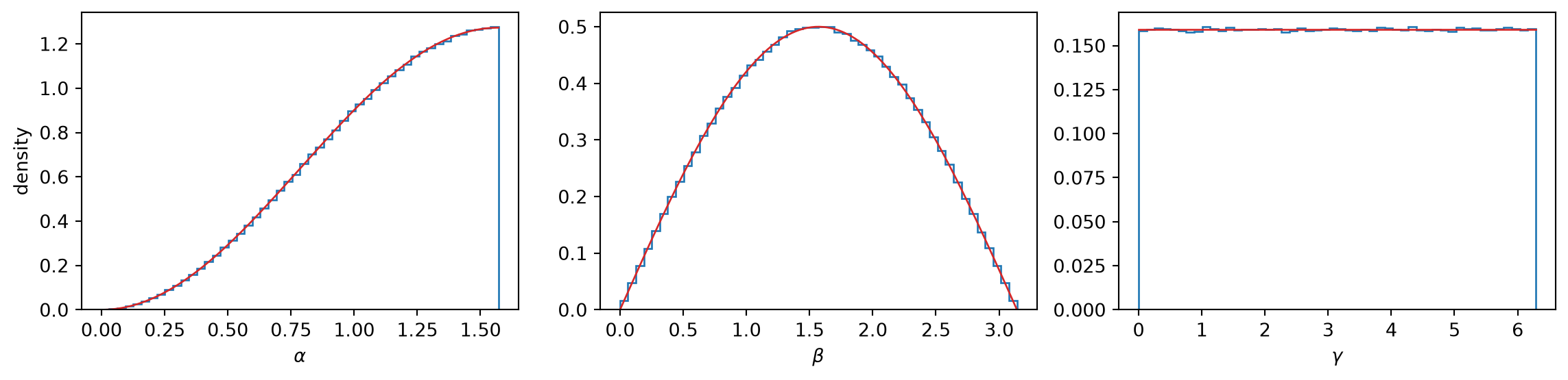
Code
# Round trip through the angles and the rotation of one vector, on random parameters.
worst_q, worst_v = 0.0, 0.0
for _ in range(200):
    u = rng.uniform(size=3)
    for i, x in enumerate(u):
        cosmo.orig_param_set(Nc.HCosmoBISParams.U1 + i, x)
    q = cosmo.get_quaternion()
    sign = -1.0 if q.s < 0.0 else 1.0
    alpha, beta, gamma = cosmo.get_angles()
    q_angles = np.array(
        [
            math.cos(alpha),
            math.sin(alpha) * math.cos(beta),
            math.sin(alpha) * math.sin(beta) * math.cos(gamma),
            math.sin(alpha) * math.sin(beta) * math.sin(gamma),
        ]
    )
    worst_q = max(worst_q, np.abs(q_angles - sign * np.array([q.s, q.v.c[0], q.v.c[1], q.v.c[2]])).max())
    v1 = Ncm.TriVec.new_full([0.36, -0.48, 0.8])
    q.rotate(v1)
    cosmo.set_angles(alpha, beta, gamma)
    v2 = Ncm.TriVec.new_full([0.36, -0.48, 0.8])
    cosmo.get_quaternion().rotate(v2)
    worst_v = max(worst_v, max(abs(v1.c[i] - v2.c[i]) for i in range(3)))
print(f"largest difference of the quaternion rebuilt from the angles: {worst_q:.1e}; of a rotated vector after set_angles: {worst_v:.1e}")
largest difference of the quaternion rebuilt from the angles: 5.3e-16; of a rotated vector after set_angles: 1.3e-15The symmetry of the axes
This symmetry is a property of the likelihood, not of the parametrization. The distance of a source depends on its direction \(\hat n\) only through \(n_1^2\), \(n_2^2\), \(n_3^2\), so it is invariant under the three reflections \(n_i \to -n_i\). The orientation is a unit quaternion, which parametrizes the proper rotations only: reflections are improper and are excluded by the parametrization itself, so they never arise in the parameter space. What the parameters inherit from the invariance is its proper part, the products of two reflections, which are the rotations by \(\pi\) about the axes. With the identity, the three rotations by \(\pi\) form the group of the symmetry that acts on the box. Each is a rotation of \(\hat n\) in the frame of the axes, \(\hat n \to g\,\hat n\,g^\dagger\) with \(g\) the unit quaternion \(i\), \(j\) or \(k\), so on the orientation it acts from the left, \[ q \to g\,q, \qquad g \in \{1, i, j, k\}, \] and together with the sign of \(q\) the orbit of an orientation has eight points, \(g \in \{\pm 1, \pm i, \pm j, \pm k\}\). The right product \(q \to q\,g\) rotates the sky direction \(\hat p\) instead and is not a symmetry.
In the complex form \(z_1 = a + id = \sqrt{u_1}\,e^{2\pi i u_3}\), \(z_2 = c + ib = \sqrt{1 - u_1}\,e^{2\pi i u_2}\), the products are \[ k\,q = (iz_1,\; -iz_2), \qquad i\,q = (iz_2,\; iz_1), \qquad -q = (-z_1,\; -z_2), \] by expanding \(k(a + bi + cj + dk)\) and \(i(a + bi + cj + dk)\). Multiplication of \(z_1\) or \(z_2\) by \(i\) is a quarter turn of its phase, a shift of \(u_3\) or \(u_2\) by \(\tfrac14\); the exchange of \(z_1\) and \(z_2\) sends \(u_1\) to \(1 - u_1\). The eight images of \((u_1, u_2, u_3)\), modulo 1, are therefore \[ k^m q:\ (u_1,\; u_2 - \tfrac{m}{4},\; u_3 + \tfrac{m}{4}), \qquad j^m i\,q:\ (1 - u_1,\; u_3 + \tfrac14 - \tfrac{m}{4},\; u_2 + \tfrac14 + \tfrac{m}{4}), \qquad m = 0, 1, 2, 3, \] where \(k^2 = j^2 = -1\) gives the sign of \(q\). The rotations by \(\pi\) of space appear as quarter turns on the box because the quaternion angle is half the rotation angle.
Fundamental domain. Within the first family \(u_1\) is fixed and \(u_2\) takes the four values \(u_2 - m/4\), one of which lies in \([0, \tfrac14)\); within the second family \(u_1\) is replaced by \(1 - u_1\) and \(u_2\) takes the four values \(u_3 + \tfrac14 - m/4\), again one in \([0, \tfrac14)\). The condition \(u_1 \leq \tfrac12\) selects one family (for \(u_1 \neq \tfrac12\)) and \(0 \leq u_2 < \tfrac14\) selects one member of it, so the domain \[ u_1 \leq \tfrac12, \qquad 0 \leq u_2 < \tfrac14 \] holds one image of every orientation. It is the domain used by the Bianchi I experiments, and it keeps the flat measure, being a subset of the box.
Reading the image from the parameters. A point \((u_1, u_2, u_3)\) belongs to the first family if \(u_1 \leq \tfrac12\), with \(m = -\lfloor 4u_2 \rfloor \bmod 4\) and representative \((u_1, u_2 + m/4, u_3 - m/4)\); otherwise to the second family, with \(m = \lfloor 4(u_3 - \tfrac14) \rfloor \bmod 4\) and representative \((1 - u_1, u_3 - \tfrac14 - m/4, u_2 - \tfrac14 + m/4)\), all modulo 1. The group element is \(k^m\) in the first family and \(j^m i\) in the second: \(1, k, -1, -k\) and \(i, j, -i, -j\) for \(m = 0, 1, 2, 3\).
A cut on the right products is not a fundamental domain. A rule that keeps \(a \geq 0\) and, among the right products \(q, qi, qj, qk\), the lexicographically largest \((a, b, c, d)\), compares \(q\) with points that are not its images. On the true orbit it keeps one, two or three of the eight images (31%, 50% and 19% of random orientations), so a posterior restricted by it keeps up to three copies of an orientation and loses part of the others.
The chunk below checks, on random orientations, that the eight left images give the same distance moduli, that the right products do not, that the representative read from the parameters lies in the domain with the stated group element, and the count of images kept by the cut on the right products.
Code
def set_quaternion(a, b, c, d):
    """Set the model's orientation from (a, b, c, d) through the axis-angle constructor."""
    norm = math.sqrt(b * b + c * c + d * d)
    q = Ncm.Quaternion.new()
    q.set_from_data(b / norm, c / norm, d / norm, 2.0 * math.atan2(norm, a))
    cosmo.set_quaternion(q)
    return np.array([cosmo.orig_param_get(Nc.HCosmoBISParams.U1 + i) for i in range(3)])


def qmul(p, r):
    a1, b1, c1, d1 = p
    a2, b2, c2, d2 = r
    return np.array(
        [
            a1 * a2 - b1 * b2 - c1 * c2 - d1 * d2,
            a1 * b2 + b1 * a2 + c1 * d2 - d1 * c2,
            a1 * c2 - b1 * d2 + c1 * a2 + d1 * b2,
            a1 * d2 + b1 * c2 - c1 * b2 + d1 * a2,
        ]
    )


UNITS = {"1": (1, 0, 0, 0), "i": (0, 1, 0, 0), "j": (0, 0, 1, 0), "k": (0, 0, 0, 1)}


def unit(name):
    return (-1.0 if name.startswith("-") else 1.0) * np.array(UNITS[name.strip("-")], float)


def classify(u):
    u1, u2, u3 = u
    if u1 <= 0.5:
        m = (-int(math.floor(4.0 * u2))) % 4
        return np.array([u1, (u2 + m / 4.0) % 1.0, (u3 - m / 4.0) % 1.0]), ["1", "k", "-1", "-k"][m]
    m = int(math.floor(4.0 * ((u3 - 0.25) % 1.0)))
    return np.array([1.0 - u1, (u3 - 0.25 - m / 4.0) % 1.0, (u2 - 0.25 + m / 4.0) % 1.0]), ["i", "j", "-i", "-j"][m]


def moduli(q):
    set_quaternion(*q)
    dist.prepare(cosmo)
    return np.array([dist.dmodulus_sky(0.05, *p) for p in directions])


def principal_right(q):
    a, b, c, d = q
    cand = np.array([[a, b, c, d], [-b, a, d, -c], [-c, -d, a, b], [-d, c, -b, a]])
    return q[0] >= 0.0 and np.allclose(cand[max(range(4), key=lambda i: tuple(cand[i]))], q)


for i, h in enumerate((0.9 * 73.0, 73.0, 1.1 * 73.0)):
    cosmo.orig_param_set(i, h)
dist = Nc.HCosmoBIDist.new(0.2)
directions = rng.normal(size=(10, 3))
directions /= np.linalg.norm(directions, axis=1)[:, None]

worst_left, best_right, n_domain, n_group = 0.0, np.inf, 0, 0
kept = np.zeros(9, int)
n_trials = 40
for _ in range(n_trials):
    u = rng.uniform(size=3)
    q = quaternion(u)
    mu = moduli(q)
    images = [s * qmul(unit(g), q) for g in ("1", "i", "j", "k") for s in (1.0, -1.0)]
    worst_left = max(worst_left, max(np.abs(moduli(img) - mu).max() for img in images))
    best_right = min(best_right, min(np.abs(moduli(qmul(q, unit(g))) - mu).max() for g in ("i", "j", "k")))
    rep, g = classify(u)
    n_domain += (rep[0] <= 0.5) and (0.0 <= rep[1] < 0.25)
    n_group += np.allclose(qmul(unit(g), quaternion(rep)), q, atol=1.0e-12)
    kept[sum(principal_right(img) for img in images)] += 1
print(f"{n_trials} orientations: moduli at the eight left images equal to {worst_left:.1e} mag; the right products differ by at least {best_right:.2f} mag")
print(f"representative in the fundamental domain: {n_domain}; q = g q_rep with the stated g: {n_group}")
print("images per orbit kept by the cut on the right products:", {k: int(v) for k, v in enumerate(kept) if v})
40 orientations: moduli at the eight left images equal to 2.8e-14 mag; the right products differ by at least 0.06 mag
representative in the fundamental domain: 40; q = g q_rep with the stated g: 40
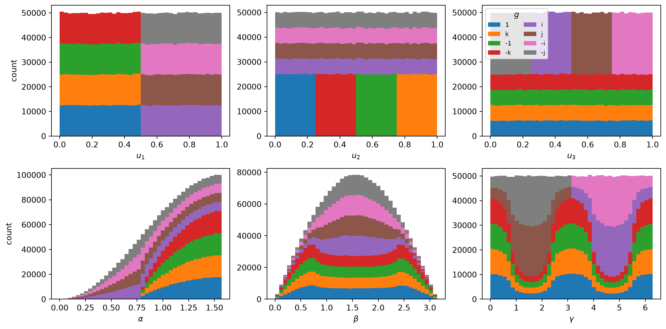
images per orbit kept by the cut on the right products: {1: 17, 2: 16, 3: 7}The classes on the draws of the box above: the eight sign patterns partition the box, and in the angles they overlap and add up to the densities of the uniform distribution.
Code
labels = ["1", "k", "-1", "-k", "i", "j", "-i", "-j"]
u1, u2, u3 = u_draws.T
first = u1 <= 0.5
m_first = (-np.floor(4.0 * u2).astype(int)) % 4
m_second = np.floor(4.0 * ((u3 - 0.25) % 1.0)).astype(int) % 4
cls = np.where(first, m_first, 4 + m_second)
colors = plt.cm.tab10(np.arange(8))

fig, axes = plt.subplots(2, 3, figsize=(12, 6))
for i, ax in enumerate(axes[0]):
    ax.hist([u_draws[cls == c, i] for c in range(8)], bins=40, range=(0, 1), stacked=True, color=colors, label=labels)
    ax.set_xlabel(f"$u_{i + 1}$")
ranges = [(0, math.pi / 2), (0, math.pi), (0, 2 * math.pi)]
names = [r"$\alpha$", r"$\beta$", r"$\gamma$"]
for i, ax in enumerate(axes[1]):
    ax.hist([angles[cls == c, i] for c in range(8)], bins=40, range=ranges[i], stacked=True, color=colors)
    ax.set_xlabel(names[i])
axes[0, 0].set_ylabel("count")
axes[1, 0].set_ylabel("count")
axes[0, 2].legend(title="$g$", ncol=2, fontsize=8)
plt.tight_layout()
plt.show()