This page describes how NcXcorKernel computes the window \(W_\ell(k)\) under the Limber approximation.
The Limber approximation is activated by NcXcorKernel:l-limber. Its value \(\ell_\mathrm{limber}\) divides the multipoles: those with \(\ell \ge \ell_\mathrm{limber}\) take the Limber path, and those below take the non-Limber path of UltraLevin: Non-Limber Angular Power Spectra. The value 0 puts every multipole on the Limber path, and -1 puts none.
The two paths differ in a single step. In both, each component of a kernel has a radial kernel \(K(\chi,k)\), its radial integral \(I_\ell(k)\) (Eq. (2) of the UltraLevin page) and a prefactor \(p_\ell(k)\), and its window is \(W_\ell(k) = p_\ell(k)\, I_\ell(k)\). The non-Limber path computes \(I_\ell(k)\) as a Levin integral; the Limber path replaces it by a closed form in \(K\). After that step the paths are the same: \(W_\ell(k)\) is represented over \(k\) as in The window over k, and a pair of windows is integrated as in The outer integral.
The Limber path also requires the radial kernel of each component to be a product of two factors, \[
K(\chi,k) = K_\chi(\chi)\, K_k(\chi,k),
\] with \(K_\chi\) a function of the distance alone and \(K_k\) the factor that depends on the wavenumber. For the galaxy clustering component of NcXcorKernelGal, \(K_k\) is \(\sqrt{P(k,z)}\) at the redshift \(z\) of \(\chi\). The component evaluates \(K_\chi\) with nc_xcor_kernel_component_eval_window, \(K_k\) with nc_xcor_kernel_component_eval_kfactor and \(p_\ell\) with nc_xcor_kernel_component_eval_prefactor. The factorization is what lets the multipoles of a block share the evaluations at one distance, as described below.
Throughout, \(\nu_m \equiv m + 1/2\) and \(\nu \equiv \nu_\ell\).
Code
import numpy as npimport matplotlib.pyplot as pltfrom matplotlib.ticker import FormatStrFormatterfrom numcosmo_py import Nc, NcmNcm.cfg_init()plt.rcParams.update({"figure.dpi": 110, "axes.grid": True, "grid.alpha": 0.3})cosmo = Nc.HICosmoDEXcdm.new()dist = Nc.Distance.new(5.0)dist.prepare(cosmo)ps = Ncm.PowspecAnalytic.new( Ncm.PowspecAnalyticShape.BBKS, Ncm.PowspecAnalyticGrowth.LCDM)def gauss_window( l_limber: int, ell: int, deriv: int=0, n_sigma: float=4.0) -> Nc.XcorKernelIntegrand:"""The window of a Gaussian kernel at one multipole, exact or under Limber.""" sbi = Ncm.SBesselIntegratorLevin.new(ell, ell) kernel = Nc.XcorKernelAnalyticGauss( dist=dist, powspec=ps, chi_mean=1500.0, chi_sigma=300.0, n_sigma=n_sigma, integrator=sbi, bessel_deriv=deriv, ) kernel.set_l_limber(l_limber) kernel.set_reltol(1.0e-8) kernel.prepare(cosmo)return kernel.get_eval_vectorized_full(cosmo, ell, ell, sbi)
The Limber form of the radial integral
The Limber approximation expands the radial integral in \(1/\nu\), assuming that \(K\) is smooth in \(\chi\); the terms beyond the leading one involve derivatives of \(K\) in \(\chi\)(Loverde and Afshordi 2008). The leading term is \(K\) at \(k\chi = \nu\) times the integral of the weight, \[
\int_0^\infty j_\ell(x)\,\mathrm{d}x = \frac{\sqrt{\pi}}{2}\,
\frac{\Gamma\big((\ell+1)/2\big)}{\Gamma\big(\ell/2+1\big)}
\simeq \sqrt{\frac{\pi}{2\nu}},
\] where the last form differs from the Gamma ratio by a relative amount of order \(1/\nu^2\) (0.9% at \(\ell = 2\), \(6 \times 10^{-6}\) at \(\ell = 100\)). For the weight \(j_m\), \[
\int \mathrm{d}\chi\, K(\chi,k)\, j_m(k\chi) \simeq I^\mathrm{L}_m(k),
\qquad
I^\mathrm{L}_m(k) \equiv \sqrt{\frac{\pi}{2\nu_m}}\,\frac{K(\nu_m / k,\, k)}{k},
\] with a relative error of order \(1/\nu_m^2\). So \(I_\ell(k) \simeq I^\mathrm{L}_\ell(k)\). The index \(m\) is general because the derivative weights below need \(I^\mathrm{L}_{\ell+1}\) as well.
\(I^\mathrm{L}_m(k)\) is \(K\) evaluated at the single distance \(\chi_m = \nu_m / k\). Since \(K\) vanishes outside its support \([\chi_\mathrm{min}, \chi_\mathrm{max}]\), \(I^\mathrm{L}_m(k)\) vanishes outside the band \[
\frac{\nu_m}{\chi_\mathrm{max}} \le k \le \frac{\nu_m}{\chi_\mathrm{min}}.
\] Where \(K\) is nonzero at an end of its support, \(I^\mathrm{L}_m\) is discontinuous at the corresponding end of the band: nonzero on one side, zero on the other.
Figure 1 shows the two windows the library builds for a Gaussian kernel, one from the Levin integral of UltraLevin: Non-Limber Angular Power Spectra and one from \(I^\mathrm{L}_\ell\). Their largest difference, relative to the peak of the window, is proportional to \(1/\nu^2\) for large \(\nu\).
Figure 1: Top: the window W_l(k) of a Gaussian kernel (mean 1500 Mpc, width 300 Mpc, cut at 4 sigma) at l = 10 and l = 100, from UltraLevin (solid) and from the Limber form (dashed, a darker shade drawn over it), each divided by the peak of the UltraLevin window; at l = 100 the two coincide to 5.6e-3 of the peak. The k range shown is where either window exceeds 1e-3 of its peak. Bottom: the largest difference between the two windows over k, divided by that peak and multiplied by nu^2. The difference is 1.26 of the peak at l = 2, 5.6e-3 at l = 100 and 6.6e-4 at l = 300; times nu^2 it tends to a constant (56 at l = 100, 60 at l = 300).
Derivative weights
A component whose Bessel weight is \(j_\ell^{(d)}\), with \(d\) the component’s bessel-deriv (1 for a Doppler-type term, 2 for redshift-space distortions), has a window that the Limber form of a single order cannot represent: the moments of \(j_\ell''\) of order zero and one vanish, so the weight acts as \(\delta''\) and the leading term of its Limber expansion is a second derivative of \(K\). The library writes the derivative instead as its exact combination of neighboring orders (Olver et al. 2026, sec. 10.51.1), \[
j_\ell' = \frac{\ell\, j_{\ell-1} - (\ell+1)\, j_{\ell+1}}{2\ell+1},
\qquad
j_\ell'' = a_\ell\, j_{\ell-2} - b_\ell\, j_\ell + c_\ell\, j_{\ell+2},
\] with \[
a_\ell = \frac{\ell(\ell-1)}{(2\ell-1)(2\ell+1)},
\qquad
b_\ell = \frac{2\ell^2+2\ell-1}{(2\ell-1)(2\ell+3)},
\qquad
c_\ell = \frac{(\ell+1)(\ell+2)}{(2\ell+1)(2\ell+3)},
\] and applies the Limber form to each order, \[
W_\ell(k) \simeq p_\ell(k) \sum_t c_{\ell,t}\, I^\mathrm{L}_{\ell+t}(k),
\] where \(c_{\ell,t}\) is the coefficient of \(j_{\ell+t}\) in the weight, \(t \in \{-1, 1\}\) for \(d = 1\) and \(t \in \{-2, 0, 2\}\) for \(d = 2\), zero for a negative order, so that \(\ell = 0\) and \(1\) need no special case. The combination is a finite difference of \(K\) across the three points \(\chi_{\ell+t} = \nu_{\ell+t}/k\), spaced by \(2/k\), which the Bessel function sets rather than the kernel’s tabulation, so the knots of the splines a kernel is built from do not enter it, where they enter a derivative of \(K\) in \(\chi\). The three-point form for \(d = 2\) is the one of Tanidis and Camera (2019).
Olver, F. W. J., A. B. Olde Daalhuis, D. W. Lozier, et al. 2026. NIST Digital Library of Mathematical Functions. Https://dlmf.nist.gov/.
Tanidis, Konstantinos, and Stefano Camera. 2019. “Developing a Unified Pipeline for Large-Scale Structure Data Analysis with Angular Power Spectra – I. The Importance of Redshift-Space Distortions for Galaxy Number Counts.”Monthly Notices of the Royal Astronomical Society 489 (3): 3385–402. https://doi.org/10.1093/mnras/stz2366.
The two-point form \(-(2\ell + \tfrac14)\,\nu^{-2}\, I^\mathrm{L}_\ell + 2(\nu+1)^{-1}
I^\mathrm{L}_{\ell+1}\), obtained from the Bessel equation at the Limber point and used by other codes, does not converge: its two terms cancel to leading order and the Limber error of each is the size of what survives, about 1.2 of the window’s peak at every multipole on the kernel of Figure 2.
In the closure each order is a term of its own, sampled in \(x = k/\nu_{\ell+t}\), so that every term of every multipole of a block shares the point \(\chi = 1/x\): one window factor and one vectorized wave-number factor per term at each sample. Before the \(k\) integrals the terms of each multipole are summed into one piecewise polynomial in \(k\), on the union of their panel edges, by rebasing each term’s series onto every cell it covers and adding the coefficients; the rebase is exact, and trailing coefficients below a hundredth of the fit’s absolute floor are dropped. The \(k\) integral of a multipole is then one product of two such polynomials, as for a single order.
Discarded border contributions
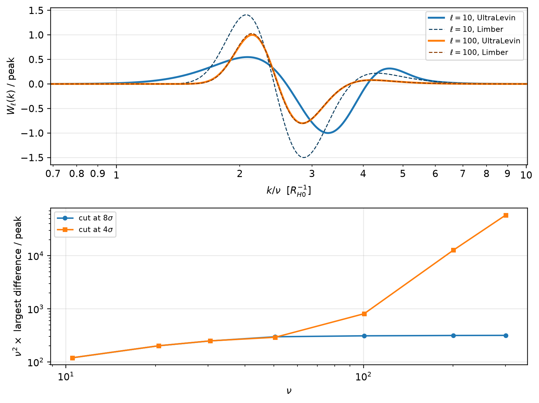
A kernel that does not vanish at an end of its support leaves a step in each order’s window at that order’s band edge, \((\nu_{\ell+t})/\chi_\mathrm{end}\), of the size of \(K\) there relative to its peak; the exact window continues past the edge as an oscillating tail of that size, which the Limber path discards, as it discards the tail of the density term at its single edge. Relative to the total window the discarded part of a derivative term is the size of the density term’s; relative to the derivative term alone it is amplified by \((\nu\sigma/\chi)^2\), \(\sigma\) the kernel’s width. Figure 2 shows both regimes. A kernel that is nonzero at its ends, or a use that needs the derivative term itself at better than that, belongs on the non-Limber path, which integrates the ends exactly.
Code
ells_d = np.array([10, 20, 30, 50, 100, 200, 300])fig, axs = plt.subplots(2, 1, figsize=(8, 6.0))q_lo, q_hi = np.inf, 0.0for ell in (10, 100): color, shade = shown[ell] levin = gauss_window(-1, ell, 2, 8.0) limber = gauss_window(0, ell, 2, 8.0) k_lo, k_hi = levin.get_range() ks = np.geomspace(k_lo, k_hi, 2000) w_levin = np.array([levin.eval_array(k)[0] for k in ks]) lo, hi = limber.get_range() w_limber = np.array([limber.eval_array(k)[0] if lo <= k <= hi else0.0for k in ks]) peak = np.abs(w_levin).max() visible = (np.abs(w_levin) >1.0e-3* peak) | (np.abs(w_limber) >1.0e-3* peak) q_lo =min(q_lo, ks[visible].min() / (ell +0.5)) q_hi =max(q_hi, ks[visible].max() / (ell +0.5)) axs[0].plot(ks / (ell +0.5), w_levin / peak, color=color, lw=2.0, label=rf"$\ell = {ell}$, UltraLevin") axs[0].plot(ks / (ell +0.5), w_limber / peak, color=shade, lw=1.0, ls="--", label=rf"$\ell = {ell}$, Limber")for n_sigma, marker in ((8.0, "o"), (4.0, "s")): scaled_d = []for ell in ells_d: levin = gauss_window(-1, ell, 2, n_sigma) limber = gauss_window(0, ell, 2, n_sigma) k_lo, k_hi = levin.get_range() ks = np.geomspace(k_lo, k_hi, 2000) w_levin = np.array([levin.eval_array(k)[0] for k in ks]) lo, hi = limber.get_range() w_limber = np.array( [limber.eval_array(k)[0] if lo <= k <= hi else0.0for k in ks] ) peak = np.abs(w_levin).max() scaled_d.append(np.abs(w_limber - w_levin).max() / peak * (ell +0.5) **2) axs[1].plot(ells_d +0.5, scaled_d, marker +"-", ms=4, label=rf"cut at ${n_sigma:g}\sigma$")axs[0].set_xscale("log")axs[0].set_xlim(q_lo, q_hi)axs[0].xaxis.set_major_formatter(FormatStrFormatter("%g"))axs[0].xaxis.set_minor_formatter(FormatStrFormatter("%g"))axs[0].set_xlabel(r"$k / \nu$[$R_{H0}^{-1}$]")axs[0].set_ylabel(r"$W_\ell(k)$ / peak")axs[0].legend(fontsize=8)axs[1].set_xscale("log")axs[1].set_yscale("log")axs[1].set_xlabel(r"$\nu$")axs[1].set_ylabel(r"$\nu^2 \times$ largest difference / peak")axs[1].legend(fontsize=8)fig.tight_layout()plt.show()
Figure 2: The window W_l(k) of the Gaussian kernel of Figure 1 with the j_l’’ weight, at l = 10 and l = 100, from UltraLevin (solid) and from the Limber form of the recurrence (dashed), each divided by the peak of the UltraLevin window; the kernel is cut at 8 sigma, where it is 1e-14 of its peak. Bottom: the largest difference between the two windows over k, divided by that peak and multiplied by nu^2, for the cut at 8 sigma (circles) and at 4 sigma (squares), where the kernel is 3e-4 of its peak at the cut: the first tends to a constant, the second grows with nu as the discarded border contributions of the three orders do.