import sys
import numpy as np
import math
import matplotlib.pyplot as plt
from IPython.display import HTML, Markdown, display

# CCL
import pyccl
import pandas as pd

# NumCosmo
from numcosmo_py import Nc, Ncm

from numcosmo_py.plotting.tools import set_rc_params_article, format_time
import numcosmo_py.cosmology as ncc
import numcosmo_py.ccl.comparison as nc_cmpBenchmarking NumCosmo vs. CCL
Abstract
This document shows the NumCosmo implementation of cosmology background functions and compares it to the CCL ones.
Introduction
This notebook explores the cosmological background functions implemented in the Core Cosmology Library (CCL) and NumCosmo, two frameworks for computing cosmological quantities. We aim to assess the consistency and accuracy of distance measures, such as comoving and luminosity distances, across these frameworks by comparing their outputs under identical physical parameters. To facilitate this analysis, we first establish a set of cosmological models with fixed and variable parameters, then define a function to compute and visualize the distances alongside their relative differences. The results are summarized in tables and plots below.
Initializing NumCosmo
To begin, we configure NumCosmo and redirect its output to this notebook using the following code:
Ncm.cfg_init()
Ncm.cfg_set_log_handler(lambda msg: sys.stdout.write(msg) and sys.stdout.flush())
set_rc_params_article(ncol=2, fontsize=12, use_tex=False)
Initial Parameter Definitions
We initialize the cosmological parameters and model-specific variables used for CCL and NumCosmo comparisons. Scalar parameters are fixed across all models, while arrays define variations in dark energy and neutrino properties for multiple scenarios. First, we instantiate a CCL cosmology object using the predefined global parameters. Next, using the numcosmo_py[^numcosmo_py] function create_nc_obj, we generate a NumCosmo cosmology object initialized with the same parameters as the CCL model. Fixed scalars apply universally, while arrays (\(\Omega_v\), \(w_0\), \(w_a\), \(m_\nu\)) represent different model configurations. Finally, in the setup_models function, one can enable high-precision computations in CCL, which increases accuracy at the cost of longer computation times. When this mode is activated, the overall agreement between CCL and NumCosmo improves significantly.
Code
from numcosmo_py.ccl.nc_ccl import create_nc_obj

PARAMETERS_SET = [
    r"$\Lambda$CDM, flat",
    r"$\Lambda$CDM, flat, $1\nu$",
    r"XCDM, flat",
    r"XCDM, spherical, $2\nu$",
    r"XCDM, hyperbolic",
]
COLORS = plt.rcParams["axes.prop_cycle"].by_key()["color"][:5]


def setup_models(
    Omega_c: float = 0.25,  # Cold dark matter density
    Omega_b: float = 0.05,  # Baryonic matter density
    h: float = 0.7,  # Dimensionless Hubble constant
    sigma8: float = 0.9,  # Matter density contrast std. dev. (8 Mpc/h)
    n_s: float = 0.96,  # Scalar spectral index
    Neff: float = 3.046,  # Effective number of massless neutrinos
    high_precision: bool = False,  # Use high precision computations in CCL
    dist_z_max: float = 15.0,  # Maximum redshift for distance computations
):
    """Setup cosmological models."""
    Omega_v_vals = np.array([0.7, 0.7, 0.7, 0.65, 0.75])  # Dark energy density
    w0_vals = np.array([-1.0, -1.0, -0.9, -0.9, -0.9])  # DE equation of state w0
    wa_vals = np.array([0.0, 0.0, 0.1, 0.1, 0.1])  # DE equation of state wa

    # Neutrino masses (eV) for each model: [m1, m2, m3]
    mnu = np.array(
        [
            [0.0, 0.0, 0.0],
            [0.04, 0.0, 0.0],
            [0.0, 0.0, 0.0],
            [0.03, 0.02, 0.0],
            [0.0, 0.0, 0.0],
        ]
    )
    Omega_k_vals = [
        float(1.0 - Omega_c - Omega_b - Omega_v) for Omega_v in Omega_v_vals
    ]

    parameters = [
        ["$\\Omega_c$", "Cold Dark Matter Density", Omega_c],
        ["$\\Omega_b$", "Baryonic Matter Density", Omega_b],
        ["$\\Omega_v$", "Dark Energy Density", Omega_v_vals],
        ["$\\Omega_k$", "Curvature Density", [f"{v:.3f}" for v in Omega_k_vals]],
        ["$h$", "Hubble Constant (dimensionless)", h],
        ["$n_s$", "Scalar Spectral Index", n_s],
        ["$N_\\mathrm{eff}$", "Effective Nº of Massless Neutrinos", Neff],
        ["$\\sigma_8$", "Matter Density Contrast Std. Dev. (8 Mpc/h)", sigma8],
        ["$w_0$", "DE Equation of State Parameter", w0_vals],
        ["$w_a$", "DE Equation of State Parameter", wa_vals],
        ["$m_\\nu$", "Neutrino Masses (eV)", [f"{m.tolist()}" for m in mnu]],
    ]
    models = []
    if high_precision:
        CCLParams.set_high_prec_params()

    for Omega_v, Omega_k, w0, wa, m in zip(
        Omega_v_vals, Omega_k_vals, w0_vals, wa_vals, mnu
    ):
        ccl_cosmo = pyccl.Cosmology(
            Omega_c=Omega_c,
            Omega_b=Omega_b,
            Neff=Neff,
            h=h,
            sigma8=sigma8,
            n_s=n_s,
            Omega_k=Omega_k,
            w0=w0,
            wa=wa,
            m_nu=m,
            transfer_function="eisenstein_hu",
        )
        cosmology = create_nc_obj(ccl_cosmo, dist_z_max=dist_z_max)
        models.append({"CCL": ccl_cosmo, "NC": cosmology})

    return parameters, models
# Preparing the models
parameters, models = setup_models(high_precision=False)
z = np.geomspace(0.01, 1200.0, 10000)Parameter Overview
The table below summarizes the parameters. There are five parameters sets.
Code
# Create DataFrame
df = pd.DataFrame(parameters, columns=["Symbol", "Description", "Value"])
display(Markdown(df.to_markdown(index=False, colalign=["left"] * len(df.columns))))| Symbol | Description | Value |
|---|---|---|
| \(\Omega_c\) | Cold Dark Matter Density | 0.25 |
| \(\Omega_b\) | Baryonic Matter Density | 0.05 |
| \(\Omega_v\) | Dark Energy Density | [0.7 0.7 0.7 0.65 0.75] |
| \(\Omega_k\) | Curvature Density | [‘0.000’, ‘0.000’, ‘0.000’, ‘0.050’, ‘-0.050’] |
| \(h\) | Hubble Constant (dimensionless) | 0.7 |
| \(n_s\) | Scalar Spectral Index | 0.96 |
| \(N_\mathrm{eff}\) | Effective Nº of Massless Neutrinos | 3.046 |
| \(\sigma_8\) | Matter Density Contrast Std. Dev. (8 Mpc/h) | 0.9 |
| \(w_0\) | DE Equation of State Parameter | [-1. -1. -0.9 -0.9 -0.9] |
| \(w_a\) | DE Equation of State Parameter | [0. 0. 0.1 0.1 0.1] |
| \(m_\nu\) | Neutrino Masses (eV) | [‘[0.0, 0.0, 0.0]’, ‘[0.04, 0.0, 0.0]’, ‘[0.0, 0.0, 0.0]’, ‘[0.03, 0.02, 0.0]’, ‘[0.0, 0.0, 0.0]’] |
Cosmology Parameters
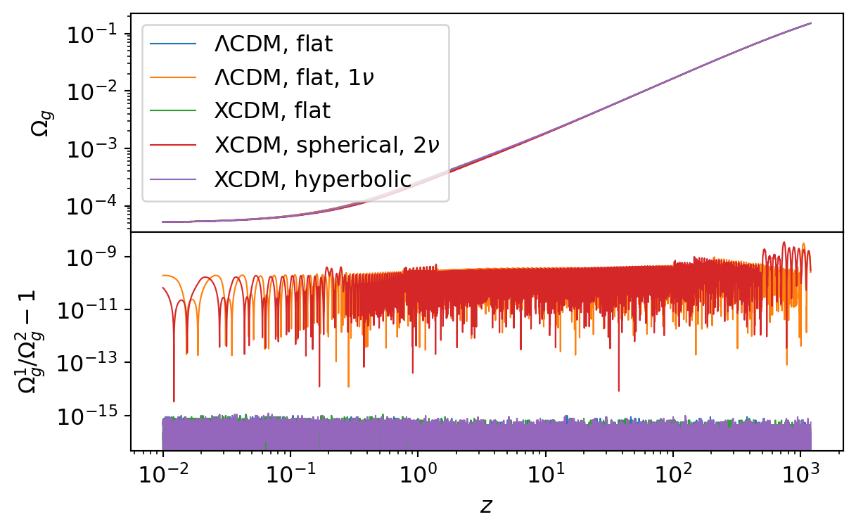
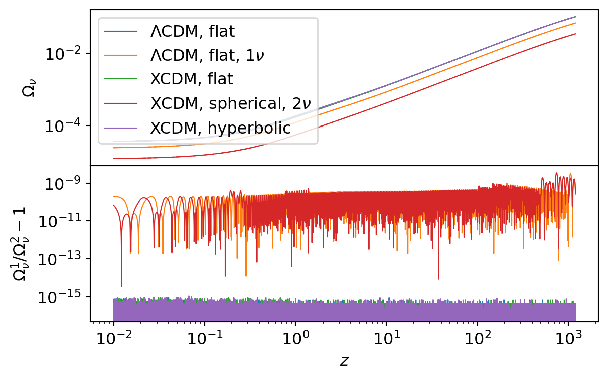
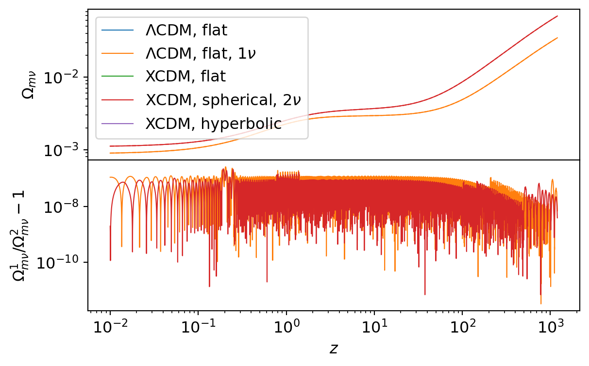
The following function compares the total mass density (baryonic + cold dark matter + massive neutrinos), the total mass density parameter, and the normalized Hubble function. Below, we present the results for all sets of parameters.
Note that in CCL, the total matter density parameter is defined as the sum of the matter density parameter and the massive neutrino density parameter. In contrast, NumCosmo defines it as the sum of the matter density parameter and the fraction of the massive neutrino density parameter that is non-relativistic at a given redshift. For consistency, we compute \(\Omega_m\) using the CCL prescription, this is done turning the CCL_comp parameter to True in the NumCosmo cosmology object.
parameter_funcs = [
    nc_cmp.compare_Omega_m,
    nc_cmp.compare_Omega_g,
    nc_cmp.compare_Omega_nu,
    nc_cmp.compare_Omega_mnu,
]

parameter_comparisons: list[list[nc_cmp.CompareFunc1d]] = [
    [func(m["CCL"], m["NC"], z, model=name) for m, name in zip(models, PARAMETERS_SET)]
    for func in parameter_funcs
]
Code
for parameter_comparison in parameter_comparisons:
    fig, axs = plt.subplots(2, sharex=True)
    fig.subplots_adjust(hspace=0)

    for p, c in zip(parameter_comparison, COLORS):
        p.xscale = "log"
        p.plot(axs=axs, color=c)

plt.show()
plt.close()
/home/runner/work/NumCosmo/NumCosmo/numcosmo_py/ccl/comparison.py:144: UserWarning: Data has no positive values, and therefore cannot be log-scaled.
axs[0].set_yscale(self.yscale)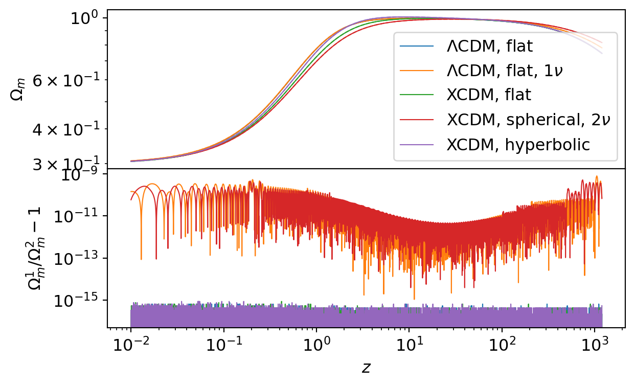
The following table summarizes the results for all sets.
Code
table = []

for parameter_comparison in parameter_comparisons:
    for p in parameter_comparison:
        table.append(p.summary_row())

df = pd.DataFrame(table, columns=nc_cmp.CompareFunc1d.table_header())

display(Markdown(df.to_markdown(index=False, colalign=["left"] * len(df.columns))))| Model | Quantity | \(\Delta P_{\text{min}}/P\) | \(\Delta P_{\text{max}}/P\) | \(\overline{\Delta P / P}\) | \(\sigma_{\Delta P / P}\) |
|---|---|---|---|---|---|
| \(\Lambda\)CDM, flat | \(\Omega_m\) | \(0\) | \(7.8 \times 10^{-16}\) | \(1.7 \times 10^{-16}\) | \(1.3 \times 10^{-16}\) |
| \(\Lambda\)CDM, flat, \(1\nu\) | \(\Omega_m\) | \(1.1 \times 10^{-15}\) | \(7.9 \times 10^{-10}\) | \(7.1 \times 10^{-11}\) | \(10^{-10}\) |
| XCDM, flat | \(\Omega_m\) | \(0\) | \(8.9 \times 10^{-16}\) | \(1.7 \times 10^{-16}\) | \(1.4 \times 10^{-16}\) |
| XCDM, spherical, \(2\nu\) | \(\Omega_m\) | \(4 \times 10^{-15}\) | \(5.2 \times 10^{-10}\) | \(6.9 \times 10^{-11}\) | \(8.6 \times 10^{-11}\) |
| XCDM, hyperbolic | \(\Omega_m\) | \(0\) | \(8.9 \times 10^{-16}\) | \(1.8 \times 10^{-16}\) | \(1.5 \times 10^{-16}\) |
| \(\Lambda\)CDM, flat | \(\Omega_g\) | \(0\) | \(10^{-15}\) | \(2.3 \times 10^{-16}\) | \(1.8 \times 10^{-16}\) |
| \(\Lambda\)CDM, flat, \(1\nu\) | \(\Omega_g\) | \(1.2 \times 10^{-14}\) | \(3.2 \times 10^{-9}\) | \(2 \times 10^{-10}\) | \(2.2 \times 10^{-10}\) |
| XCDM, flat | \(\Omega_g\) | \(0\) | \(1.1 \times 10^{-15}\) | \(2.4 \times 10^{-16}\) | \(1.9 \times 10^{-16}\) |
| XCDM, spherical, \(2\nu\) | \(\Omega_g\) | \(3.3 \times 10^{-15}\) | \(3.5 \times 10^{-9}\) | \(2.3 \times 10^{-10}\) | \(3.4 \times 10^{-10}\) |
| XCDM, hyperbolic | \(\Omega_g\) | \(0\) | \(1.2 \times 10^{-15}\) | \(2.5 \times 10^{-16}\) | \(1.9 \times 10^{-16}\) |
| \(\Lambda\)CDM, flat | \(\Omega_{\nu}\) | \(0\) | \(8.9 \times 10^{-16}\) | \(1.9 \times 10^{-16}\) | \(1.6 \times 10^{-16}\) |
| \(\Lambda\)CDM, flat, \(1\nu\) | \(\Omega_{\nu}\) | \(1.2 \times 10^{-14}\) | \(3.2 \times 10^{-9}\) | \(2 \times 10^{-10}\) | \(2.2 \times 10^{-10}\) |
| XCDM, flat | \(\Omega_{\nu}\) | \(0\) | \(8.9 \times 10^{-16}\) | \(2 \times 10^{-16}\) | \(1.6 \times 10^{-16}\) |
| XCDM, spherical, \(2\nu\) | \(\Omega_{\nu}\) | \(3.6 \times 10^{-15}\) | \(3.5 \times 10^{-9}\) | \(2.3 \times 10^{-10}\) | \(3.4 \times 10^{-10}\) |
| XCDM, hyperbolic | \(\Omega_{\nu}\) | \(0\) | \(1.1 \times 10^{-15}\) | \(2.1 \times 10^{-16}\) | \(1.7 \times 10^{-16}\) |
| \(\Lambda\)CDM, flat | \(\Omega_{m\nu}\) | \(0\) | \(0\) | \(0\) | \(0\) |
| \(\Lambda\)CDM, flat, \(1\nu\) | \(\Omega_{m\nu}\) | \(3.2 \times 10^{-12}\) | \(2.7 \times 10^{-7}\) | \(6.6 \times 10^{-8}\) | \(4.3 \times 10^{-8}\) |
| XCDM, flat | \(\Omega_{m\nu}\) | \(0\) | \(0\) | \(0\) | \(0\) |
| XCDM, spherical, \(2\nu\) | \(\Omega_{m\nu}\) | \(6.7 \times 10^{-12}\) | \(2.3 \times 10^{-7}\) | \(4.5 \times 10^{-8}\) | \(3.3 \times 10^{-8}\) |
| XCDM, hyperbolic | \(\Omega_{m\nu}\) | \(0\) | \(0\) | \(0\) | \(0\) |
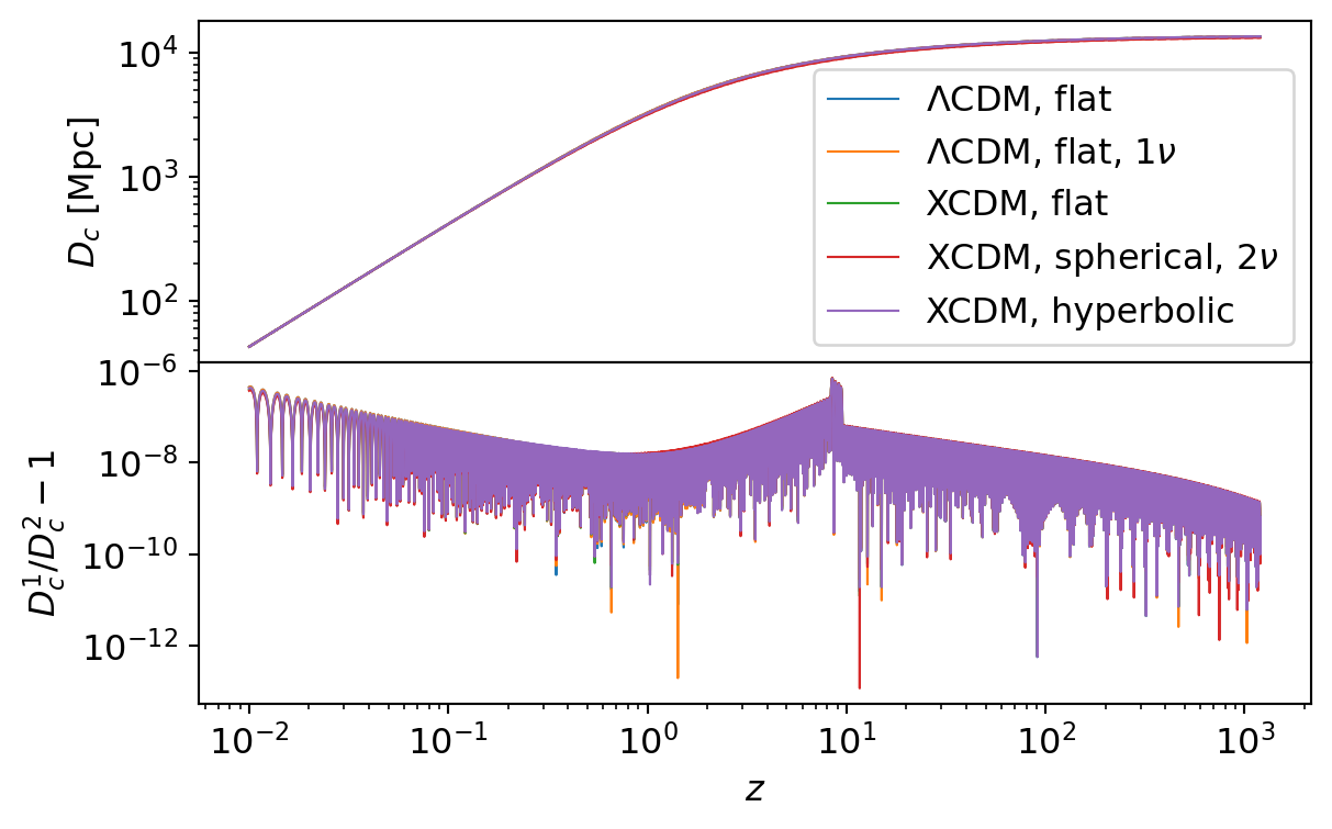
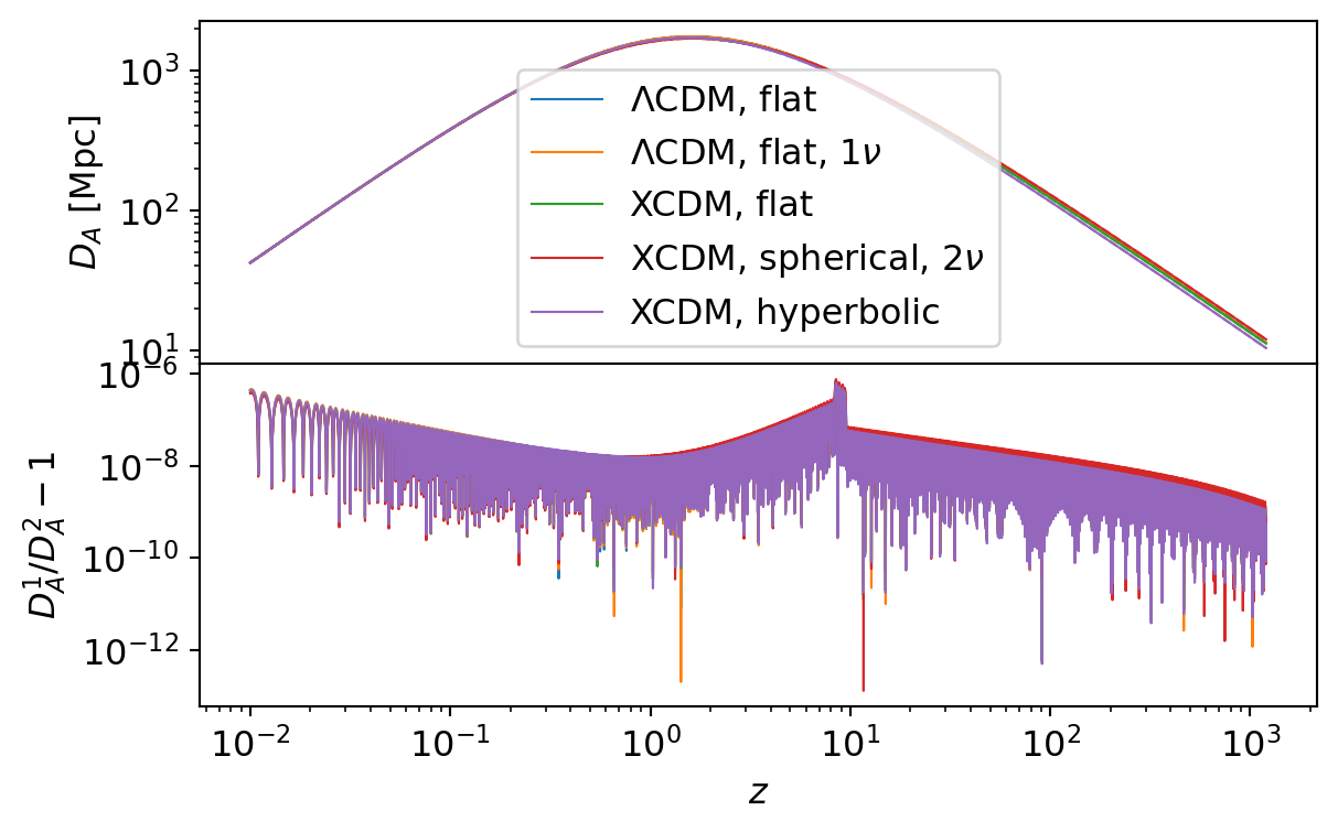
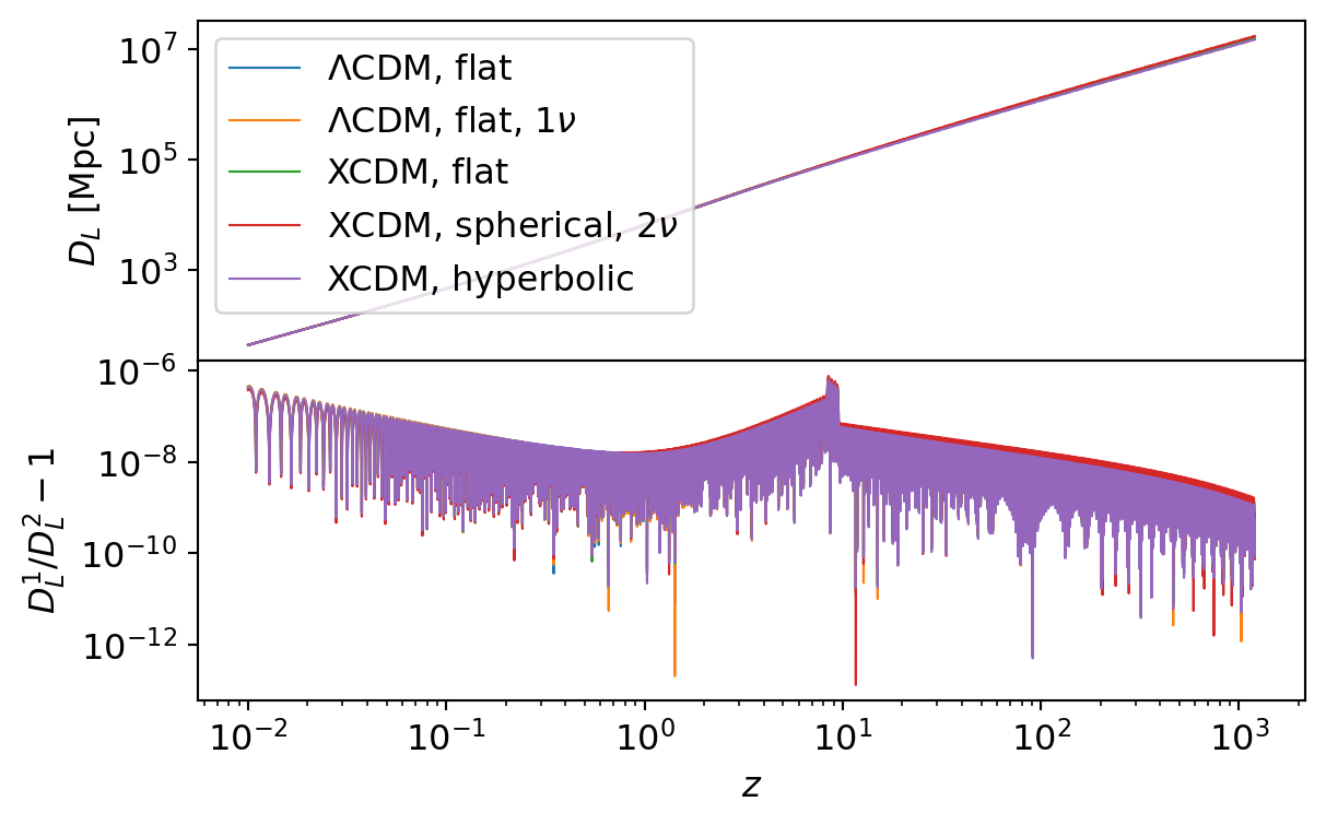
Distances
We define a function to compare cosmological distances calculated by the CCL and NumCosmo frameworks. The function then evaluates and compares the cosmological distances implemented in both libraries. Expand the cell below to view the code.
distance_funcs = [
nc_cmp.compare_Hubble,
nc_cmp.compare_distance_comoving,
nc_cmp.compare_distance_transverse,
nc_cmp.compare_distance_angular_diameter,
nc_cmp.compare_distance_luminosity,
nc_cmp.compare_distance_modulus,
nc_cmp.compare_distance_lookback_time,
nc_cmp.compare_distance_comoving_volume,
]
distance_comparisons: list[list[nc_cmp.CompareFunc1d]] = [
[func(m["CCL"], m["NC"], z, model=name) for m, name in zip(models, PARAMETERS_SET)]
for func in distance_funcs
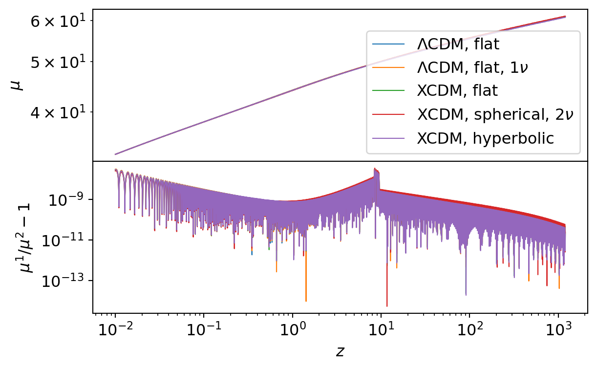
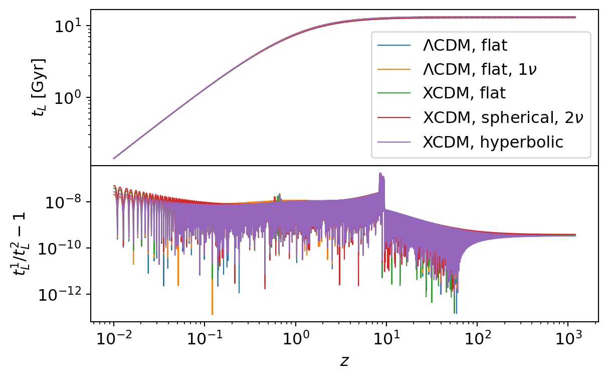
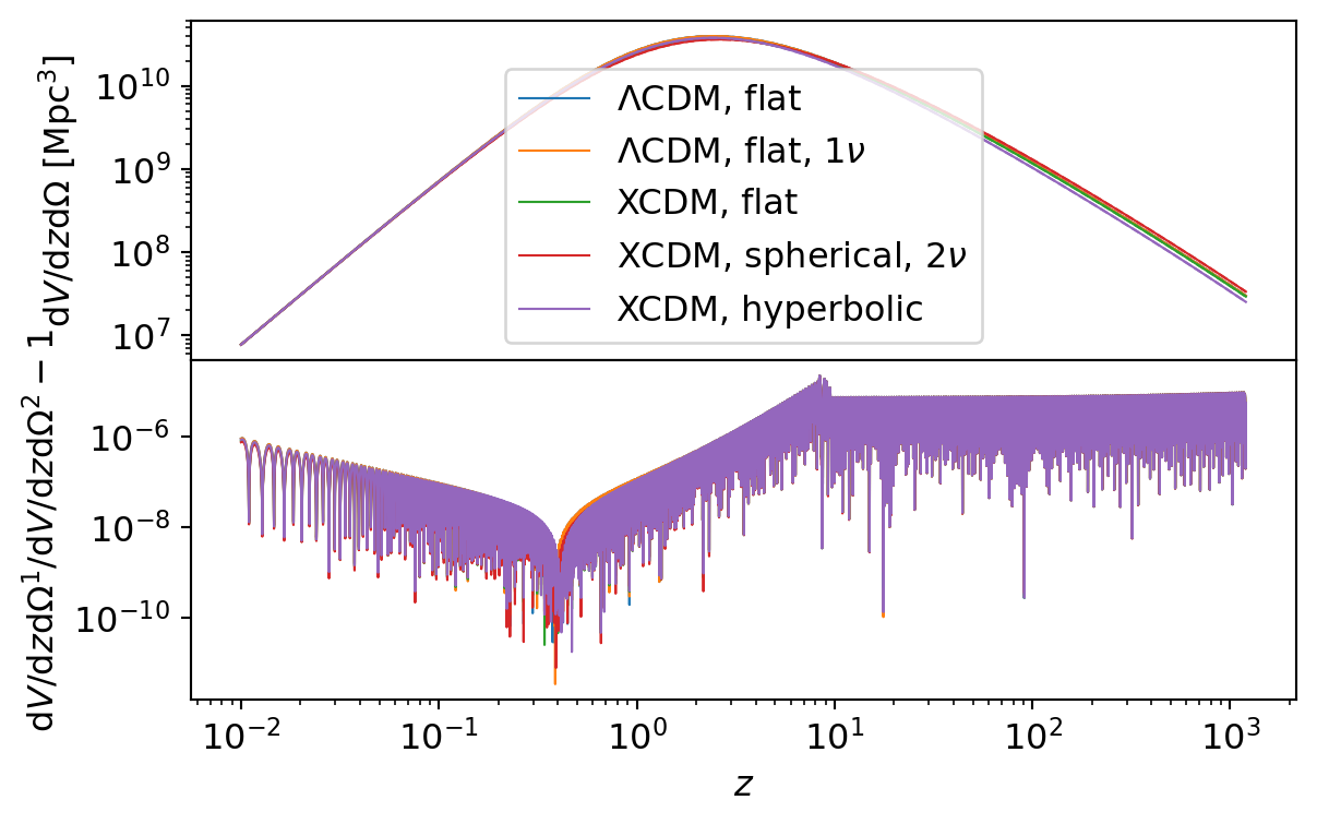
]We plot the distance comparisons for all parameter sets.
Code
for distance_comparison in distance_comparisons:
    fig, axs = plt.subplots(2, sharex=True)
    fig.subplots_adjust(hspace=0)

    for d, c in zip(distance_comparison, COLORS):
        d.xscale = "log"
        d.plot(axs=axs, color=c)

plt.show()
plt.close()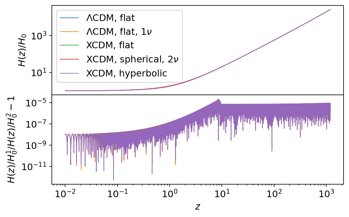

Again a table summarizes the results for all parameter sets.
Code
table = []

for distance_comparison in distance_comparisons:
    for d in distance_comparison:
        table.append(d.summary_row())

df = pd.DataFrame(table, columns=nc_cmp.CompareFunc1d.table_header())

display(Markdown(df.to_markdown(index=False, colalign=["left"] * len(df.columns))))| Model | Quantity | \(\Delta P_{\text{min}}/P\) | \(\Delta P_{\text{max}}/P\) | \(\overline{\Delta P / P}\) | \(\sigma_{\Delta P / P}\) |
|---|---|---|---|---|---|
| \(\Lambda\)CDM, flat | \(H(z)/H_0\) | \(3.2 \times 10^{-12}\) | \(2.3 \times 10^{-5}\) | \(2.5 \times 10^{-6}\) | \(3.1 \times 10^{-6}\) |
| \(\Lambda\)CDM, flat, \(1\nu\) | \(H(z)/H_0\) | \(4.5 \times 10^{-12}\) | \(2.3 \times 10^{-5}\) | \(2.5 \times 10^{-6}\) | \(3.1 \times 10^{-6}\) |
| XCDM, flat | \(H(z)/H_0\) | \(5.1 \times 10^{-13}\) | \(2.3 \times 10^{-5}\) | \(2.5 \times 10^{-6}\) | \(3.1 \times 10^{-6}\) |
| XCDM, spherical, \(2\nu\) | \(H(z)/H_0\) | \(1.5 \times 10^{-11}\) | \(2.2 \times 10^{-5}\) | \(2.5 \times 10^{-6}\) | \(3.1 \times 10^{-6}\) |
| XCDM, hyperbolic | \(H(z)/H_0\) | \(1.8 \times 10^{-12}\) | \(2.3 \times 10^{-5}\) | \(2.5 \times 10^{-6}\) | \(3.1 \times 10^{-6}\) |
| \(\Lambda\)CDM, flat | \(D_c\) [Mpc] | \(5.8 \times 10^{-13}\) | \(6.8 \times 10^{-7}\) | \(4.5 \times 10^{-8}\) | \(7.8 \times 10^{-8}\) |
| \(\Lambda\)CDM, flat, \(1\nu\) | \(D_c\) [Mpc] | \(2 \times 10^{-13}\) | \(6.8 \times 10^{-7}\) | \(4.5 \times 10^{-8}\) | \(7.8 \times 10^{-8}\) |
| XCDM, flat | \(D_c\) [Mpc] | \(5.9 \times 10^{-13}\) | \(7 \times 10^{-7}\) | \(4.3 \times 10^{-8}\) | \(7.3 \times 10^{-8}\) |
| XCDM, spherical, \(2\nu\) | \(D_c\) [Mpc] | \(1.2 \times 10^{-13}\) | \(7.1 \times 10^{-7}\) | \(4.2 \times 10^{-8}\) | \(7.1 \times 10^{-8}\) |
| XCDM, hyperbolic | \(D_c\) [Mpc] | \(5.8 \times 10^{-13}\) | \(6.8 \times 10^{-7}\) | \(4.4 \times 10^{-8}\) | \(7.5 \times 10^{-8}\) |
| \(\Lambda\)CDM, flat | \(D_t\) [Mpc] | \(5.8 \times 10^{-13}\) | \(6.8 \times 10^{-7}\) | \(4.5 \times 10^{-8}\) | \(7.8 \times 10^{-8}\) |
| \(\Lambda\)CDM, flat, \(1\nu\) | \(D_t\) [Mpc] | \(2 \times 10^{-13}\) | \(6.8 \times 10^{-7}\) | \(4.5 \times 10^{-8}\) | \(7.8 \times 10^{-8}\) |
| XCDM, flat | \(D_t\) [Mpc] | \(5.9 \times 10^{-13}\) | \(7 \times 10^{-7}\) | \(4.3 \times 10^{-8}\) | \(7.3 \times 10^{-8}\) |
| XCDM, spherical, \(2\nu\) | \(D_t\) [Mpc] | \(1.3 \times 10^{-13}\) | \(7.6 \times 10^{-7}\) | \(4.3 \times 10^{-8}\) | \(7.4 \times 10^{-8}\) |
| XCDM, hyperbolic | \(D_t\) [Mpc] | \(5 \times 10^{-13}\) | \(6.3 \times 10^{-7}\) | \(4.3 \times 10^{-8}\) | \(7.3 \times 10^{-8}\) |
| \(\Lambda\)CDM, flat | \(D_A\) [Mpc] | \(5.8 \times 10^{-13}\) | \(6.8 \times 10^{-7}\) | \(4.5 \times 10^{-8}\) | \(7.8 \times 10^{-8}\) |
| \(\Lambda\)CDM, flat, \(1\nu\) | \(D_A\) [Mpc] | \(2 \times 10^{-13}\) | \(6.8 \times 10^{-7}\) | \(4.5 \times 10^{-8}\) | \(7.8 \times 10^{-8}\) |
| XCDM, flat | \(D_A\) [Mpc] | \(5.9 \times 10^{-13}\) | \(7 \times 10^{-7}\) | \(4.3 \times 10^{-8}\) | \(7.3 \times 10^{-8}\) |
| XCDM, spherical, \(2\nu\) | \(D_A\) [Mpc] | \(1.3 \times 10^{-13}\) | \(7.6 \times 10^{-7}\) | \(4.3 \times 10^{-8}\) | \(7.4 \times 10^{-8}\) |
| XCDM, hyperbolic | \(D_A\) [Mpc] | \(5 \times 10^{-13}\) | \(6.3 \times 10^{-7}\) | \(4.3 \times 10^{-8}\) | \(7.3 \times 10^{-8}\) |
| \(\Lambda\)CDM, flat | \(D_L\) [Mpc] | \(5.8 \times 10^{-13}\) | \(6.8 \times 10^{-7}\) | \(4.5 \times 10^{-8}\) | \(7.8 \times 10^{-8}\) |
| \(\Lambda\)CDM, flat, \(1\nu\) | \(D_L\) [Mpc] | \(2 \times 10^{-13}\) | \(6.8 \times 10^{-7}\) | \(4.5 \times 10^{-8}\) | \(7.8 \times 10^{-8}\) |
| XCDM, flat | \(D_L\) [Mpc] | \(5.9 \times 10^{-13}\) | \(7 \times 10^{-7}\) | \(4.3 \times 10^{-8}\) | \(7.3 \times 10^{-8}\) |
| XCDM, spherical, \(2\nu\) | \(D_L\) [Mpc] | \(1.3 \times 10^{-13}\) | \(7.6 \times 10^{-7}\) | \(4.3 \times 10^{-8}\) | \(7.4 \times 10^{-8}\) |
| XCDM, hyperbolic | \(D_L\) [Mpc] | \(5 \times 10^{-13}\) | \(6.3 \times 10^{-7}\) | \(4.3 \times 10^{-8}\) | \(7.3 \times 10^{-8}\) |
| \(\Lambda\)CDM, flat | \(\mu\) | \(2.3 \times 10^{-14}\) | \(3 \times 10^{-8}\) | \(2.5 \times 10^{-9}\) | \(4.5 \times 10^{-9}\) |
| \(\Lambda\)CDM, flat, \(1\nu\) | \(\mu\) | \(9.8 \times 10^{-15}\) | \(3 \times 10^{-8}\) | \(2.5 \times 10^{-9}\) | \(4.5 \times 10^{-9}\) |
| XCDM, flat | \(\mu\) | \(2.3 \times 10^{-14}\) | \(3.1 \times 10^{-8}\) | \(2.3 \times 10^{-9}\) | \(4.1 \times 10^{-9}\) |
| XCDM, spherical, \(2\nu\) | \(\mu\) | \(5.6 \times 10^{-15}\) | \(3.3 \times 10^{-8}\) | \(2.3 \times 10^{-9}\) | \(4 \times 10^{-9}\) |
| XCDM, hyperbolic | \(\mu\) | \(2 \times 10^{-14}\) | \(2.8 \times 10^{-8}\) | \(2.3 \times 10^{-9}\) | \(4.2 \times 10^{-9}\) |
| \(\Lambda\)CDM, flat | \(t_L\) [Gyr] | \(1.4 \times 10^{-13}\) | \(1.8 \times 10^{-7}\) | \(5.5 \times 10^{-9}\) | \(1.1 \times 10^{-8}\) |
| \(\Lambda\)CDM, flat, \(1\nu\) | \(t_L\) [Gyr] | \(1.3 \times 10^{-13}\) | \(1.8 \times 10^{-7}\) | \(5.5 \times 10^{-9}\) | \(1.1 \times 10^{-8}\) |
| XCDM, flat | \(t_L\) [Gyr] | \(1.5 \times 10^{-13}\) | \(1.8 \times 10^{-7}\) | \(6.3 \times 10^{-9}\) | \(1.2 \times 10^{-8}\) |
| XCDM, spherical, \(2\nu\) | \(t_L\) [Gyr] | \(1.3 \times 10^{-12}\) | \(1.7 \times 10^{-7}\) | \(6.8 \times 10^{-9}\) | \(1.3 \times 10^{-8}\) |
| XCDM, hyperbolic | \(t_L\) [Gyr] | \(9.6 \times 10^{-13}\) | \(1.8 \times 10^{-7}\) | \(5.7 \times 10^{-9}\) | \(1.2 \times 10^{-8}\) |
| \(\Lambda\)CDM, flat | \(\mathrm{d}V/\mathrm{d}z\mathrm{d}\Omega\) [Mpc\({}^3\)] | \(2.8 \times 10^{-11}\) | \(2.2 \times 10^{-5}\) | \(2.5 \times 10^{-6}\) | \(3 \times 10^{-6}\) |
| \(\Lambda\)CDM, flat, \(1\nu\) | \(\mathrm{d}V/\mathrm{d}z\mathrm{d}\Omega\) [Mpc\({}^3\)] | \(3.5 \times 10^{-12}\) | \(2.1 \times 10^{-5}\) | \(2.5 \times 10^{-6}\) | \(3 \times 10^{-6}\) |
| XCDM, flat | \(\mathrm{d}V/\mathrm{d}z\mathrm{d}\Omega\) [Mpc\({}^3\)] | \(2.5 \times 10^{-11}\) | \(2.1 \times 10^{-5}\) | \(2.5 \times 10^{-6}\) | \(3 \times 10^{-6}\) |
| XCDM, spherical, \(2\nu\) | \(\mathrm{d}V/\mathrm{d}z\mathrm{d}\Omega\) [Mpc\({}^3\)] | \(7.9 \times 10^{-12}\) | \(2.1 \times 10^{-5}\) | \(2.5 \times 10^{-6}\) | \(3 \times 10^{-6}\) |
| XCDM, hyperbolic | \(\mathrm{d}V/\mathrm{d}z\mathrm{d}\Omega\) [Mpc\({}^3\)] | \(1.8 \times 10^{-11}\) | \(2.2 \times 10^{-5}\) | \(2.5 \times 10^{-6}\) | \(3.1 \times 10^{-6}\) |
Time Comparison
We compare the time spent on calculating the cosmological distances. First, it is necessary to create again the cosmology used in the function, then we use “timeit” to estimate the mean time intervals it takes for each library to perform the calculations. Below we show the comparison using the first set of parameters.
Code
def compute_distance_times(
    ccl_cosmo: pyccl.Cosmology, cosmology: ncc.Cosmology, z: np.ndarray
):
    cosmo = cosmology.cosmo
    dist = cosmology.dist

    a = 1.0 / (1.0 + z)
    z_vec = Ncm.Vector.new_array(z)
    D_vec = z_vec.dup()
    table = [
        ["Comoving Distance", "CCL"]
        + nc_cmp.compute_times(lambda: pyccl.comoving_radial_distance(ccl_cosmo, a)),
        ["Comoving Distance", "NumCosmo"]
        + nc_cmp.compute_times(lambda: dist.comoving_vector(cosmo, z_vec, D_vec)),
        ["Transverse Distance", "CCL"]
        + nc_cmp.compute_times(lambda: pyccl.comoving_angular_distance(ccl_cosmo, a)),
        ["Transverse Distance", "NumCosmo"]
        + nc_cmp.compute_times(lambda: dist.transverse_vector(cosmo, z_vec, D_vec)),
        ["Angular Diameter Distance", "CCL"]
        + nc_cmp.compute_times(lambda: pyccl.angular_diameter_distance(ccl_cosmo, a)),
        ["Angular Diameter Distance", "NumCosmo"]
        + nc_cmp.compute_times(
            lambda: dist.angular_diameter_vector(cosmo, z_vec, D_vec)
        ),
        ["Luminosity Distance", "CCL"]
        + nc_cmp.compute_times(lambda: pyccl.luminosity_distance(ccl_cosmo, a)),
        ["Luminosity Distance", "NumCosmo"]
        + nc_cmp.compute_times(lambda: dist.luminosity_vector(cosmo, z_vec, D_vec)),
        ["Distance Modulus", "CCL"]
        + nc_cmp.compute_times(lambda: pyccl.distance_modulus(ccl_cosmo, a)),
        ["Distance Modulus", "NumCosmo"]
        + nc_cmp.compute_times(lambda: dist.dmodulus_vector(cosmo, z_vec, D_vec)),
    ]
    columns = ["Distance", "Library", "Mean Time", "Standard Deviation"]
    df = pd.DataFrame(table, columns=columns)

    df["Mean Time"] = df["Mean Time"].apply(format_time)
    df["Standard Deviation"] = df["Standard Deviation"].apply(format_time)
    return df


df = compute_distance_times(models[0]["CCL"], models[0]["NC"], z)

display(Markdown(df.to_markdown(index=False, colalign=["left"] * len(df.columns))))| Distance | Library | Mean Time | Standard Deviation |
|---|---|---|---|
| Comoving Distance | CCL | 179.02 \(\mu\)s | 17.62 \(\mu\)s |
| Comoving Distance | NumCosmo | 1.35 ms | 1.43 \(\mu\)s |
| Transverse Distance | CCL | 232.56 \(\mu\)s | 1.35 \(\mu\)s |
| Transverse Distance | NumCosmo | 1.36 ms | 6.05 \(\mu\)s |
| Angular Diameter Distance | CCL | 350.41 \(\mu\)s | 417.95 ns |
| Angular Diameter Distance | NumCosmo | 1.39 ms | 47.96 \(\mu\)s |
| Luminosity Distance | CCL | 232.51 \(\mu\)s | 1.45 \(\mu\)s |
| Luminosity Distance | NumCosmo | 1.36 ms | 5.84 \(\mu\)s |
| Distance Modulus | CCL | 331.34 \(\mu\)s | 1.05 \(\mu\)s |
| Distance Modulus | NumCosmo | 1.51 ms | 2.05 \(\mu\)s |
Growth Factor and Growth Rate
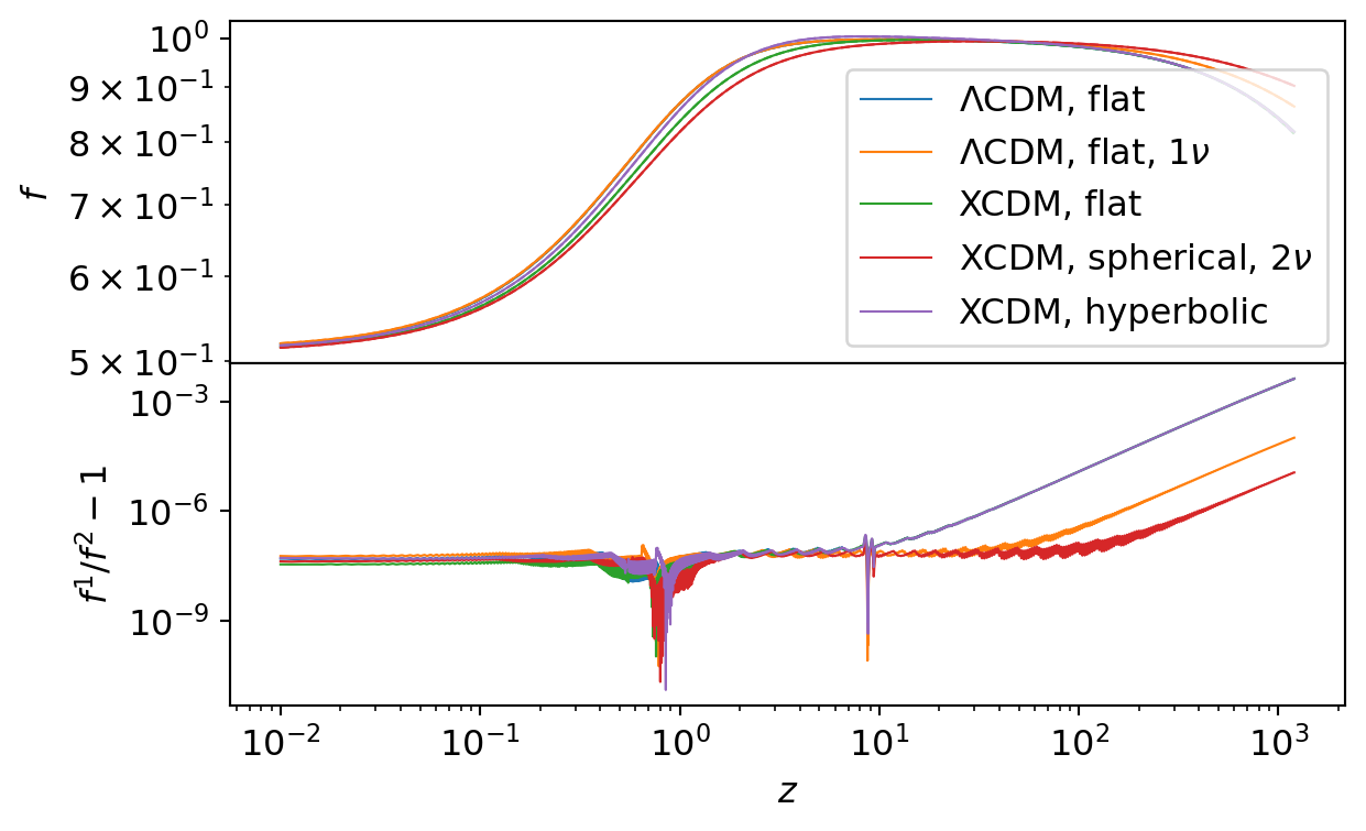
The following function compares the growth factor and growth rate between the CCL and NumCosmo cosmologies.
Since CCL defines \(\Omega_m\) differently from NumCosmo, the resulting growth factor and growth rate will also differ. In practice, CCL includes ultra-relativistic neutrinos in the matter density, leading to increasing deviations at higher redshifts when compared to NumCosmo. However, since we are using the CCL_comp mode of NumCosmo, we compute \(\Omega_m\) using the CCL prescription.
growth_funcs = [
    nc_cmp.compare_growth_factor,
    nc_cmp.compare_growth_rate,
]

growth_comparisons: list[list[nc_cmp.CompareFunc1d]] = [
    [func(m["CCL"], m["NC"], z, model=name) for m, name in zip(models, PARAMETERS_SET)]
    for func in growth_funcs
]
Below we plot the growth comparisons for all parameter sets.
Code
for growth_comparison in growth_comparisons:
    fig, axs = plt.subplots(2, sharex=True)
    fig.subplots_adjust(hspace=0)

    for p, c in zip(growth_comparison, COLORS):
        p.xscale = "log"
        p.plot(axs=axs, color=c)

plt.show()
plt.close()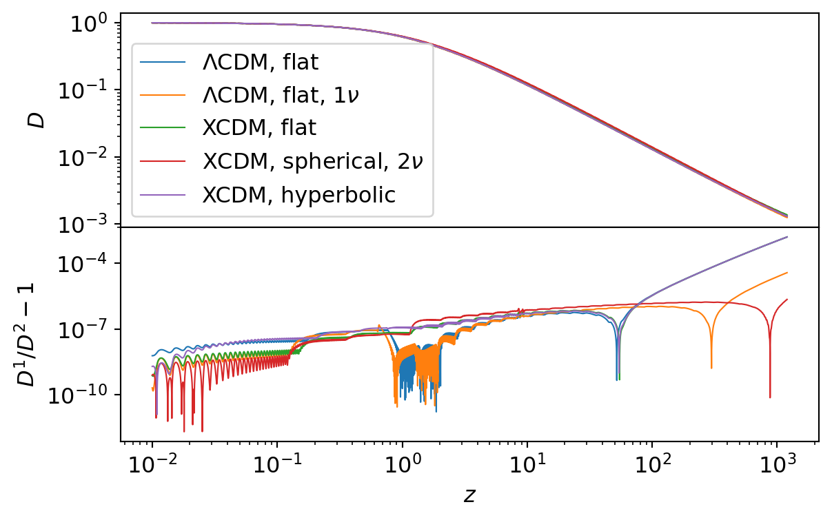
The following table summarizes the results for all sets.
Code
table = []

for growth_comparison in growth_comparisons:
    for d in growth_comparison:
        table.append(d.summary_row(convert_g=False))

df = pd.DataFrame(table, columns=nc_cmp.CompareFunc1d.table_header())
display(Markdown(df.to_markdown(index=False, colalign=["left"] * len(df.columns))))| Model | Quantity | \(\Delta P_{\text{min}}/P\) | \(\Delta P_{\text{max}}/P\) | \(\overline{\Delta P / P}\) | \(\sigma_{\Delta P / P}\) |
|---|---|---|---|---|---|
| \(\Lambda\)CDM, flat | \(D\) | \(1.67 \times 10^{-11}\) | \(1.61 \times 10^{-3}\) | \(6.15 \times 10^{-5}\) | \(2.17 \times 10^{-4}\) |
| \(\Lambda\)CDM, flat, \(1\nu\) | \(D\) | \(2.77 \times 10^{-11}\) | \(3.79 \times 10^{-5}\) | \(1.50 \times 10^{-6}\) | \(4.82 \times 10^{-6}\) |
| XCDM, flat | \(D\) | \(4.92 \times 10^{-10}\) | \(1.61 \times 10^{-3}\) | \(6.15 \times 10^{-5}\) | \(2.16 \times 10^{-4}\) |
| XCDM, spherical, \(2\nu\) | \(D\) | \(2.07 \times 10^{-12}\) | \(2.27 \times 10^{-6}\) | \(5.98 \times 10^{-7}\) | \(6.17 \times 10^{-7}\) |
| XCDM, hyperbolic | \(D\) | \(1.26 \times 10^{-11}\) | \(1.61 \times 10^{-3}\) | \(6.15 \times 10^{-5}\) | \(2.16 \times 10^{-4}\) |
| \(\Lambda\)CDM, flat | \(f\) | \(4.80 \times 10^{-10}\) | \(4.22 \times 10^{-3}\) | \(1.60 \times 10^{-4}\) | \(5.63 \times 10^{-4}\) |
| \(\Lambda\)CDM, flat, \(1\nu\) | \(f\) | \(5.50 \times 10^{-11}\) | \(1.02 \times 10^{-4}\) | \(3.86 \times 10^{-6}\) | \(1.35 \times 10^{-5}\) |
| XCDM, flat | \(f\) | \(1.02 \times 10^{-10}\) | \(4.22 \times 10^{-3}\) | \(1.60 \times 10^{-4}\) | \(5.63 \times 10^{-4}\) |
| XCDM, spherical, \(2\nu\) | \(f\) | \(2.06 \times 10^{-11}\) | \(1.13 \times 10^{-5}\) | \(4.73 \times 10^{-7}\) | \(1.49 \times 10^{-6}\) |
| XCDM, hyperbolic | \(f\) | \(1.24 \times 10^{-11}\) | \(4.22 \times 10^{-3}\) | \(1.60 \times 10^{-4}\) | \(5.63 \times 10^{-4}\) |
Scale Factor
The next function will compare the scale factor calculated from a comoving distance \(\chi\) (in Mpc).
chi = np.geomspace(1.0e-2, 4.0e3, 1000)

compare_scale_factor: list[nc_cmp.CompareFunc1d] = [
    nc_cmp.compare_scale_factor(m["CCL"], m["NC"], chi, model=name)
    for m, name in zip(models, PARAMETERS_SET)
]
Below we compare the scale factors for all parameter sets.
Code
fig, axs = plt.subplots(2, sharex=True)
fig.subplots_adjust(hspace=0)

for p, c in zip(compare_scale_factor, COLORS):
    p.plot(axs=axs, color=c)

plt.show()
plt.close()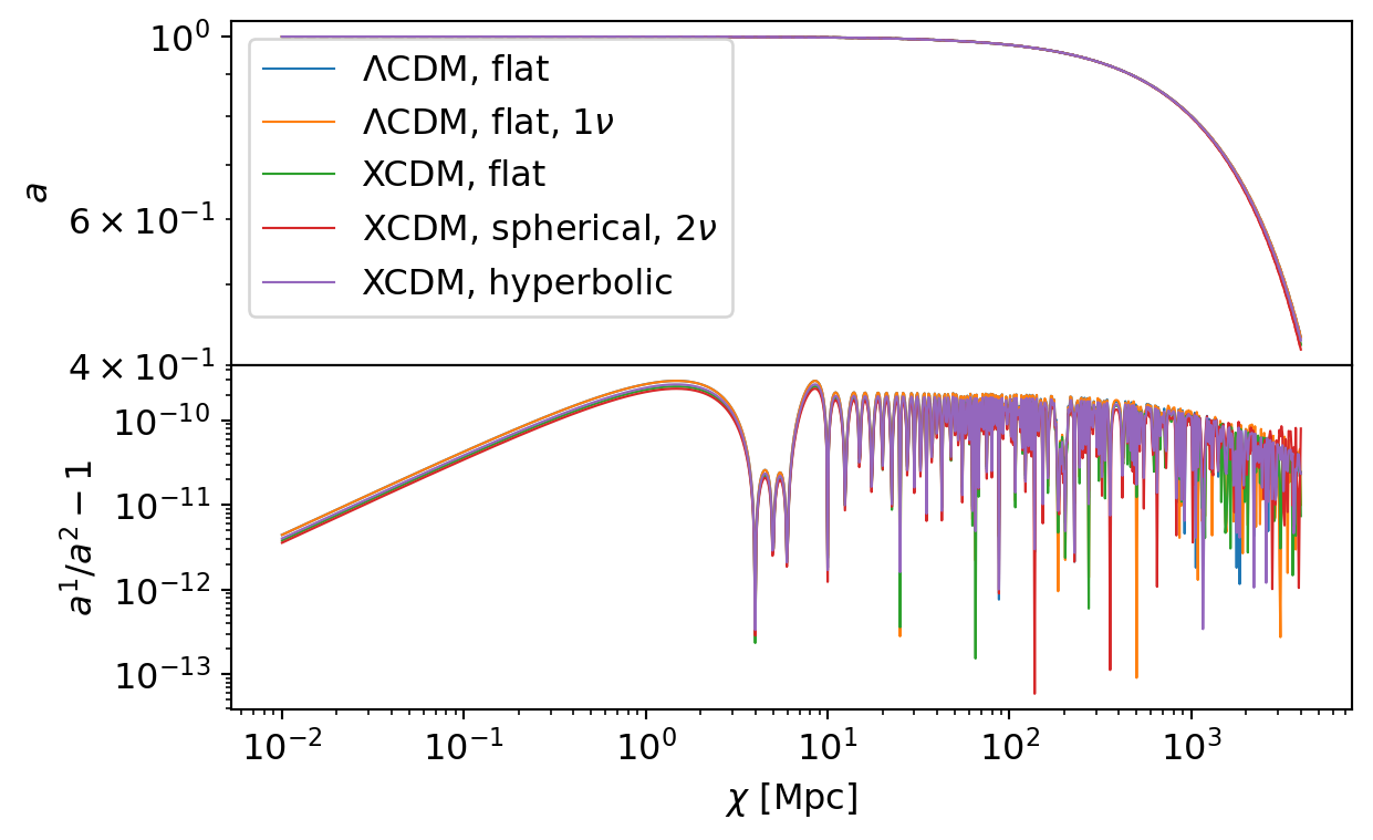
The following table summarizes the results for all sets.
Code
table = []

for d in compare_scale_factor:
    table.append(d.summary_row())

df = pd.DataFrame(table, columns=nc_cmp.CompareFunc1d.table_header())

display(Markdown(df.to_markdown(index=False, colalign=["left"] * len(df.columns))))| Model | Quantity | \(\Delta P_{\text{min}}/P\) | \(\Delta P_{\text{max}}/P\) | \(\overline{\Delta P / P}\) | \(\sigma_{\Delta P / P}\) |
|---|---|---|---|---|---|
| \(\Lambda\)CDM, flat | \(a\) | \(4 \times 10^{-13}\) | \(2.9 \times 10^{-10}\) | \(1.1 \times 10^{-10}\) | \(8.5 \times 10^{-11}\) |
| \(\Lambda\)CDM, flat, \(1\nu\) | \(a\) | \(9.1 \times 10^{-14}\) | \(2.9 \times 10^{-10}\) | \(1.1 \times 10^{-10}\) | \(8.5 \times 10^{-11}\) |
| XCDM, flat | \(a\) | \(1.5 \times 10^{-13}\) | \(2.5 \times 10^{-10}\) | \(9.3 \times 10^{-11}\) | \(7.3 \times 10^{-11}\) |
| XCDM, spherical, \(2\nu\) | \(a\) | \(5.9 \times 10^{-14}\) | \(2.4 \times 10^{-10}\) | \(8.8 \times 10^{-11}\) | \(6.8 \times 10^{-11}\) |
| XCDM, hyperbolic | \(a\) | \(3.3 \times 10^{-13}\) | \(2.6 \times 10^{-10}\) | \(9.8 \times 10^{-11}\) | \(7.7 \times 10^{-11}\) |
Critical Surface Mass Density
The next function will compare the critical surface mass density.
zs = z = np.linspace(1.0, 5.0, 10000)
zl = 0.5

compare_sigmaC: list[nc_cmp.CompareFunc1d] = [
    nc_cmp.compare_Sigma_crit(m["CCL"], m["NC"], zs, zl, model=name)
    for m, name in zip(models, PARAMETERS_SET)
]
Below we compare the critical surface mass density for all parameter sets.
Code
fig, axs = plt.subplots(2, sharex=True)
fig.subplots_adjust(hspace=0)

for p, c in zip(compare_sigmaC, COLORS):
    p.plot(axs=axs, color=c)

plt.show()
plt.close()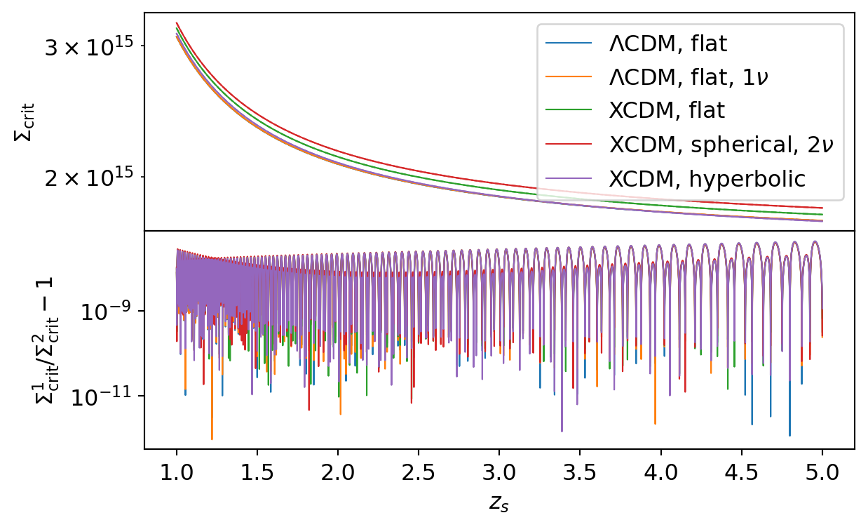
The following table summarizes the results for all sets.
Code
table = []

for d in compare_sigmaC:
    table.append(d.summary_row())

df = pd.DataFrame(table, columns=nc_cmp.CompareFunc1d.table_header())

display(Markdown(df.to_markdown(index=False, colalign=["left"] * len(df.columns))))| Model | Quantity | \(\Delta P_{\text{min}}/P\) | \(\Delta P_{\text{max}}/P\) | \(\overline{\Delta P / P}\) | \(\sigma_{\Delta P / P}\) |
|---|---|---|---|---|---|
| \(\Lambda\)CDM, flat | \(\Sigma_\mathrm{crit}\) | \(1.2 \times 10^{-12}\) | \(4.1 \times 10^{-8}\) | \(1.4 \times 10^{-8}\) | \(9.7 \times 10^{-9}\) |
| \(\Lambda\)CDM, flat, \(1\nu\) | \(\Sigma_\mathrm{crit}\) | \(9.6 \times 10^{-13}\) | \(4.1 \times 10^{-8}\) | \(1.4 \times 10^{-8}\) | \(9.7 \times 10^{-9}\) |
| XCDM, flat | \(\Sigma_\mathrm{crit}\) | \(8.5 \times 10^{-12}\) | \(4.3 \times 10^{-8}\) | \(1.4 \times 10^{-8}\) | \(10^{-8}\) |
| XCDM, spherical, \(2\nu\) | \(\Sigma_\mathrm{crit}\) | \(4.7 \times 10^{-12}\) | \(4.2 \times 10^{-8}\) | \(1.5 \times 10^{-8}\) | \(9.9 \times 10^{-9}\) |
| XCDM, hyperbolic | \(\Sigma_\mathrm{crit}\) | \(1.5 \times 10^{-12}\) | \(4.3 \times 10^{-8}\) | \(1.4 \times 10^{-8}\) | \(10^{-8}\) |
Summary
In this notebook, we compared the cosmological results obtained using CCL and NumCosmo across several sections.
- Cosmology Parameters: We examined the differences in the parameters, noting how the definitions of \(\Omega_m\) and the inclusion of massive neutrinos affect the results.
- Distances: We compared cosmological distances and found strong agreement between CCL and NumCosmo.
- Time Comparison: A detailed analysis of time measurements confirmed this consistency.
- Growth Factor and Growth Rate: We highlighted the discrepancies in the growth factor and growth rate due to CCL’s inclusion of the full neutrino energy density, which leads to increased deviations at higher redshifts.
- Scale Factor: The scale factor was also compared, showing similar trends across both methods.
- Critical Surface Mass Density: We assessed this observable and observed agreement.
Overall, the results demonstrate good agreement between the two methods, with the main differences arising from CCL’s handling of neutrinos in the background model, particularly affecting growth-related observables at higher redshifts.