Simple Cosmological Distances Example

Introduction

This example demonstrates how to compute cosmological distances using the numcosmo library. In this example, we initialize the library, configure a cosmological model, and compute comoving distances for a range of redshifts.

Prerequisites

Before running this example, make sure the numcosmo_py¹ package is installed in your environment. If it is not already installed, follow the installation instructions in the NumCosmo documentation. In addition, we are using numpy, matplotlib and pandas for data manipulation and plotting. If you are using the conda installation, these packages are already installed.

¹ NumCosmo is a C library for cosmology and astrophysics that uses GObject-Introspection to provide bindings for various programming languages. To improve the user interface, we provide a Python package, numcosmo_py. This package imports all NumCosmo bindings and includes additional helper functions to simplify library usage.

Import and Initialize

First, import the required modules and initialize the NumCosmo library. We also import numpy, matplotlib and pandas. The Nc and Ncm modules provide the core functionality of the NumCosmo library. The call to Ncm.cfg_init() initializes the library objects.

import numpy as np
import pandas as pd
import matplotlib.pyplot as plt

from numcosmo_py import Nc, Ncm

# Initialize the library objects
Ncm.cfg_init()

Set Up the Cosmological Model

Create a homogeneous and isotropic cosmological model (NcHICosmoDEXcdm) with one massive neutrino, and apply a reparameterization suitable for CMB-based parameters.

# Initialize a cosmological model
cosmo = Nc.HICosmoDEXcdm(massnu_length=1)

# Set reparameterization
cosmo.set_reparam(Nc.HICosmoDEReparamCMB.new(cosmo.len()))

Configure the Distance Calculator

Create a Distance object optimized for redshift calculations up to 2.0.

# Initialize the distance calculator
dist = Nc.Distance.new(2.0)

Set Cosmological Parameters

Assign values to the cosmological model parameters. The dictionary-based approach is used below. This approach always uses the current parameterization.

# Set parameters using original parameterization
h = 0.70
cosmo["H0"] = 100.0 * h
cosmo["omegac"] = 0.25 * h**2
cosmo["omegab"] = 0.05 * h**2
cosmo["Omegak"] = 0.0
cosmo["Tgamma0"] = 2.72
cosmo["w"] = -1.10
cosmo["massnu_0"] = 0.06

Alternatively, you can use the property-based approach to set the parameters. However, this approach always refers to the original parameterization.

# Set parameters using object-oriented style
cosmo.props.H0 = 70.00
cosmo.props.Omegab = 0.04
cosmo.props.Omegac = 0.25
cosmo.props.Omegax = 0.70
cosmo.props.Tgamma0 = 2.72
cosmo.props.w = -1.10

# Set neutrino mass vector
massnu = Ncm.Vector.new_array([0.06])
cosmo.props.massnu = massnu

Log and Prepare the Model

Log the parameter values and prepare the distance calculator for use. The calculator objects like Distance must be prepared before use.

# Log all parameters
print("# Model parameters: ")
params = cosmo.param_names()

for param in params:
    print(f"{param} = {cosmo[param]}")

# Prepare the distance calculations
dist.prepare(cosmo)

# Model parameters: 
H0 = 70.0
omegac = 0.12249999999999998
Omegak = 0.008608553079476389
Tgamma0 = 2.72
Yp = 0.24
ENnu = 3.046
omegab = 0.0196
w = -1.1
massnu_0 = 0.06
Tnu_0 = 0.71611
munu_0 = 0.0
gnu_0 = 1.0

Compute and Display Distances

Calculate and display comoving distances for a range of redshifts.

# Number of redshift steps
N = 20

# Comoving distance scaling factor
RH_Mpc = cosmo.RH_Mpc()

# Compute distances
z_array = np.linspace(0.0, 1.0, N)
Dc_array = np.array([dist.comoving(cosmo, z) for z in z_array])
dc_array = RH_Mpc * Dc_array / (1.0 + z_array)

# Putting everything in a pandas DataFrame

pd.DataFrame(
    {
        "Redshift": z_array,
        "Comoving Distance [c/H0]": Dc_array,
        "Comoving Distance [Mpc]": dc_array,
    }
)

	Redshift	Comoving Distance [c/H0]	Comoving Distance [Mpc]
0	0.000000	0.000000	0.000000
1	0.052632	0.052144	212.153565
2	0.105263	0.103255	400.100017
3	0.157895	0.153259	566.863471
4	0.210526	0.202095	714.995760
5	0.263158	0.249718	846.672769
6	0.315789	0.296098	963.766547
7	0.368421	0.341215	1067.900012
8	0.421053	0.385060	1160.489042
9	0.473684	0.427636	1242.775345
10	0.526316	0.468953	1315.852532
11	0.578947	0.509026	1380.687116
12	0.631579	0.547880	1438.135690
13	0.684211	0.585540	1488.959171
14	0.736842	0.622037	1533.834771
15	0.789474	0.657404	1573.366163
16	0.842105	0.691676	1608.092202
17	0.894737	0.724889	1638.494457
18	0.947368	0.757078	1665.003765
19	1.000000	0.788281	1688.005960

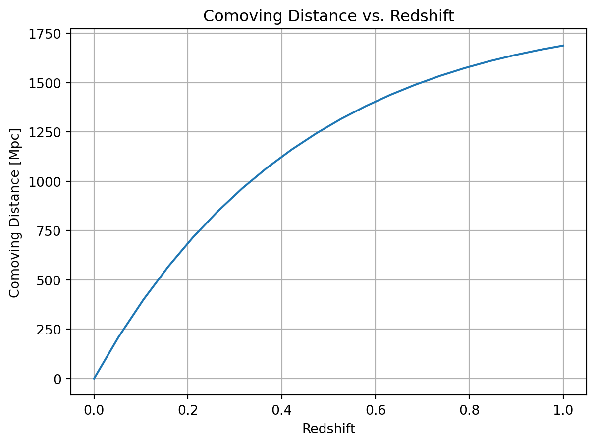
Plot the Results

You can plot the results using a plotting library such as matplotlib.

plt.plot(z_array, dc_array)
plt.xlabel("Redshift")
plt.ylabel("Comoving Distance [Mpc]")
plt.title("Comoving Distance vs. Redshift")
plt.grid()
plt.show()

Figure 1: Comoving distance vs. redshift.