def doc_theme():
    return theme_minimal() + theme(
        panel_grid_minor=element_line(color="gray", linetype="--"),
)Computing Bounce Adiabatic Spectrum
Purpose
This tutorial demonstrates how to compute the power spectrum of a bouncing cosmology using NumCosmo. A bouncing cosmology modifies the standard \(\Lambda\)CDM model by introducing a bounce, typically arising from quantum cosmology effects.
We compute and compare the power spectrum of a bouncing cosmology with that of standard \(\Lambda\)CDM. Two models are considered:
1. Single-fluid model – A single component with an arbitrary equation of state, usually interpreted as dark matter.
2. Two-fluid model – A combination of radiation and a fluid with an arbitrary equation of state (typically dark matter).
In both cases we are considering only adiabatic perturbations, see the tutorial Bounce Spectra for a more general treatment including entropy perturbations.
Defining Theoretical Models
We begin by defining a cosmological model using NumCosmo’s numcosmo_py1. Additionally, we import numpy, pandas and matplotlib, which will be used later in the tutorial.
1 NumCosmo is a C library for cosmology and astrophysics that uses GObject-Introspection to provide bindings for various programming languages. To improve the user interface, we provide a Python package, numcosmo_py. This package imports all NumCosmo bindings and includes additional helper functions to simplify library usage.
import os
import numpy as np
import pandas as pd
import matplotlib.pyplot as plt
import matplotlib.cm as cm
import matplotlib.colors as colors
from IPython.display import HTML, Markdown, display

from numcosmo_py import Nc, Ncm
from numcosmo_py.plotting.tools import (
    set_rc_params_article,
    latex_float,
    format_alpha_xaxis,
)

Ncm.cfg_init()

cosmo_w = Nc.HICosmoQGW.new()
cosmo_rw = Nc.HICosmoQGRW.new()

cosmo_w["w"] = 3.0e-19  # Set the dark energy equation of state
cosmo_rw["w"] = 3.0e-19  # Set the dark energy equation of state

cosmo_w["xb"] = 1.0e31  # Set bounce depth
cosmo_rw["xb"] = 1.0e31  # Set bounce depth

cosmo_w["Omegaw"] = 1.0  # Set dark matter fraction
cosmo_rw["Omegar"] = 1.41e-7  # Set radiation fraction
cosmo_rw["Omegaw"] = 1.0 - cosmo_rw["Omegar"]  # Set dark matter fraction

# Create bouncing/figures directory if it doesn't exist and set a variable for it
fig_dir = "bounce/figures"
if not os.path.exists(fig_dir):
    os.makedirs(fig_dir)
Model Parameters
The table below lists the parameters of the HICosmoQGW and HICosmoQGRW models.
HICosmoQGW: A single-fluid model, where QGW stands for quantum gravity with w.
HICosmoQGRW: A two-fluid model, where QGRW stands for quantum gravity with radiation and w.
Code
desc_keys = [
    "name",
    "symbol",
    "value",
    "scale",
    "abstol",
    "lower-bound",
    "upper-bound",
    "fit",
]

all_parameters = set(cosmo_w.param_names()).union(cosmo_rw.param_names())
param_data = []
for name in sorted(all_parameters):

    if name in cosmo_w.param_names():
        row = {"Parameter": f"QGW:{name}"}
        p_desc = cosmo_w.param_get_desc(name)
        for key in desc_keys:
            row[key.capitalize()] = (
                p_desc[key] if key != "symbol" else f"${p_desc[key]}$"
            )
        param_data.append(row)

    if name in cosmo_rw.param_names():
        row = {"Parameter": f"QGRW:{name}"}
        p_desc = cosmo_rw.param_get_desc(name)
        for key in desc_keys:
            row[key.capitalize()] = (
                p_desc[key] if key != "symbol" else f"${p_desc[key]}$"
            )
        param_data.append(row)


def format_column(col):
    return col.apply(lambda x: f"${latex_float(x, precision=4)}$")


df = pd.DataFrame(param_data)
df["Value"] = format_column(df["Value"])
df["Scale"] = format_column(df["Scale"])
df["Abstol"] = format_column(df["Abstol"])
df["Lower-bound"] = format_column(df["Lower-bound"])
df["Upper-bound"] = format_column(df["Upper-bound"])

display(Markdown(df.to_markdown(index=False, colalign=["left"] * len(df.columns))))| Parameter | Name | Symbol | Value | Scale | Abstol | Lower-bound | Upper-bound | Fit |
|---|---|---|---|---|---|---|---|---|
| QGW:H0 | H0 | \(H_0\) | \(67.36\) | \(1\) | \(0\) | \(10\) | \(500\) | False |
| QGRW:H0 | H0 | \(H_0\) | \(67.36\) | \(1\) | \(0\) | \(10\) | \(500\) | False |
| QGRW:Omegar | Omegar | \(\Omega_{r0}\) | \(1.41 \times 10^{-7}\) | \(0.01\) | \(0\) | \(10^{-8}\) | \(10\) | False |
| QGW:Omegaw | Omegaw | \(\Omega_{w0}\) | \(1\) | \(0.01\) | \(0\) | \(10^{-8}\) | \(10\) | False |
| QGRW:Omegaw | Omegaw | \(\Omega_{w0}\) | \(1\) | \(0.01\) | \(0\) | \(10^{-8}\) | \(10\) | False |
| QGW:w | w | \(w\) | \(3 \times 10^{-19}\) | \(10^{-8}\) | \(0\) | \(10^{-50}\) | \(1\) | False |
| QGRW:w | w | \(w\) | \(3 \times 10^{-19}\) | \(10^{-8}\) | \(0\) | \(10^{-50}\) | \(1\) | False |
| QGW:xb | xb | \(x_b\) | \(10^{31}\) | \(10^{25}\) | \(0\) | \(10^{10}\) | \(10^{40}\) | False |
| QGRW:xb | xb | \(x_b\) | \(10^{31}\) | \(10^{25}\) | \(0\) | \(10^{10}\) | \(10^{40}\) | False |
In the perturbation code, all distances are measured in units of the Hubble radius. The model evolves from \(\alpha = -\infty\) (the distant past) to \(\alpha = 0\) (the bounce). The time parameter \(\alpha\) is defined as \[ x \equiv \frac{a_0}{a} = x_b e^{-|\alpha|} \] where \(x_b\) (listed in the table above) represents the maximum contraction before the bounce.
To set up the model, we must specify the time limits, which are critical when initializing the perturbations. In practice, these limits are used to determine when the mode is accurately described by the adiabatic approximation2, a condition required to define the adiabatic vacuum. Once the initial conditions are set, the system can be numerically evolved beyond this approximation.
2 The term adiabatic appears in two distinct contexts: Adiabatic mode in perturbations: The variable \(\zeta\) describes the overall curvature perturbation, which represents a specific combination of all matter fields. In contrast, entropy modes capture the differences between individual matter fields; Adiabatic regime during evolution: At early times, each mode evolves through a phase where it is well approximated by the WKB (Wentzel-Kramers-Brillouin) method. This phase is referred to as the adiabatic regime for that perturbation.
Computing the Power Spectrum
To compute the power spectrum, we use the HIPertAdiab object, which describes the \(\zeta\) perturbation. Here, we specifically use it to identify the adiabatic regime in the sense of the WKB approximation.
# Time conversion functions
def tau_of_alpha(alpha):
    """Converts alpha to tau"""
    return np.sign(alpha) * np.acosh(
        (cosmo_rw["xb"] / cosmo_rw.eval_x(alpha)) ** (3.0 * (1.0 - cosmo_rw["w"]) / 2.0)
    )


def alpha_of_tau(tau):
    """Converts tau to alpha"""
    x = cosmo_w.eval_x(tau)
    return cosmo_rw.abs_alpha(x) * np.sign(tau)


# Compute the Hubble radius in Mpc
RH_Mpc = cosmo_w.RH_Mpc()

# Create an adiabatic perturbation object
adiab_w = Nc.HIPertAdiab.new()
adiab_rw = Nc.HIPertAdiab.new()

# Set the mode k to 1 Mpc^-1 (normalized by the Hubble radius)
k = RH_Mpc
# Set the relative tolerance for the adiabatic approximation
reltol = 5.0e-5

# Define the initial and final time limits for evolution
alpha_ini = -230.0  # Initial time in alpha
tau_ini = tau_of_alpha(alpha_ini)  # Initial time in tau

alpha_adiab_max = -1.0e-1  # Maximum time for adiabatic vacuum
tau_adiab_max = tau_of_alpha(alpha_adiab_max)

alpha_end = 20.0  # Final time in alpha
tau_end = tau_of_alpha(alpha_end)  # Final time in tau

adiab_w.set_k(k)
adiab_rw.set_k(k)

adiab_w.set_ti(tau_ini)
adiab_w.set_tf(tau_end)

adiab_rw.set_ti(alpha_ini)
adiab_rw.set_tf(alpha_end)

# Set parameters for finding the adiabatic regime
#  - Maximum time for adiabatic vacuum
#  - Relative tolerance for adiabatic approximation
adiab_w.set_vacuum_max_time(tau_adiab_max)
adiab_w.set_vacuum_reltol(reltol)

adiab_rw.set_vacuum_max_time(alpha_adiab_max)
adiab_rw.set_vacuum_reltol(reltol)

# Find the adiabatic time limit: the maximum time where the adiabatic
# approximation holds within reltol
limit_found_w, t_adiab_w = adiab_w.find_adiab_time_limit(
    cosmo_w, tau_ini, tau_end, reltol
)
limit_found_rw, t_adiab_rw = adiab_rw.find_adiab_time_limit(
    cosmo_rw, alpha_ini, alpha_end, reltol
)

# Find the adiabatic maximum: the time where the adiabatic approximation
# best describes the mode. Returns lower and upper bounds where the
# approximation deviates by 1e-1
t_min_w, F1_min_w, t_lb_w, t_ub_w = adiab_w.find_adiab_max(
    cosmo_w, tau_ini, tau_end, 1.0e-1
)
t_min_rw, F1_min_rw, t_lb_rw, t_ub_rw = adiab_rw.find_adiab_max(
    cosmo_rw, alpha_ini, alpha_end, 1.0e-1
)
We show the results in the table below:
Code
# Store results in a DataFrame for better visualization
df_adiab = pd.DataFrame(
    {
        "Parameter": [
            "Adiabatic Time Limit Found",
            "Adiabatic Time (t_adiab)",
            "Adiabatic Maximum Time (t_min)",
            "Function Value at t_min (F1_min)",
            "Lower Bound (t_lb)",
            "Upper Bound (t_ub)",
        ],
        "QGW": [
            limit_found_w,
            f"${latex_float(cosmo_w.eval_x(t_adiab_w), precision=3)}$",
            f"${latex_float(cosmo_w.eval_x(t_min_w), precision=3)}$",
            f"${latex_float(F1_min_w, precision=3)}$",
            f"${latex_float(cosmo_w.eval_x(t_lb_w), precision=3)}$",
            f"${latex_float(cosmo_w.eval_x(t_ub_w), precision=3)}$",
        ],
        "QGRW": [
            limit_found_rw,
            f"${latex_float(cosmo_rw.eval_x(t_adiab_rw), precision=3)}$",
            f"${latex_float(cosmo_rw.eval_x(t_min_rw), precision=3)}$",
            f"${latex_float(F1_min_rw, precision=3)}$",
            f"${latex_float(cosmo_rw.eval_x(t_lb_rw), precision=3)}$",
            f"${latex_float(cosmo_rw.eval_x(t_ub_rw), precision=3)}$",
        ],
    }
)

# Print the DataFrame
display(Markdown(df_adiab.to_markdown(index=False)))| Parameter | QGW | QGRW |
|---|---|---|
| Adiabatic Time Limit Found | True | True |
| Adiabatic Time (t_adiab) | \(6.72 \times 10^{-14}\) | \(6.57 \times 10^{-14}\) |
| Adiabatic Maximum Time (t_min) | \(1.29 \times 10^{-69}\) | \(1.29 \times 10^{-69}\) |
| Function Value at t_min (F1_min) | \(-1.48 \times 10^{-29}\) | \(-1.48 \times 10^{-29}\) |
| Lower Bound (t_lb) | \(1.29 \times 10^{-69}\) | \(1.29 \times 10^{-69}\) |
| Upper Bound (t_ub) | \(5.94 \times 10^{-14}\) | \(5.98 \times 10^{-14}\) |
Note that for these models, the adiabatic approximation becomes more accurate as we move further into the past \(\alpha \to -\infty\). Consequently, the best approximation is obtained at the lower bound of the time interval.
Evolving one mode
We now evolve the mode beginning at the adiabatic vacuum up to close to the bounce.
state = Ncm.CSQ1DState.new()

adiab_w.set_save_evol(True)
adiab_w.set_reltol(1.0e-10)
adiab_w.set_abstol(0.0)
adiab_w.set_initial_condition_type(Ncm.CSQ1DInitialStateType.ADIABATIC4)

adiab_w.prepare(cosmo_w)
tau_a, _ = adiab_w.get_time_array()
field_sol_w = np.array(
    [
        np.array(adiab_w.eval_at(cosmo_w, tau, state).get_phi_Pphi()).flatten()
        for tau in tau_a
    ]
)
alpha_tau_a = np.array([alpha_of_tau(tau) for tau in tau_a])

adiab_rw.set_save_evol(True)
adiab_rw.set_reltol(1.0e-10)
adiab_rw.set_abstol(0.0)
adiab_rw.set_initial_condition_type(Ncm.CSQ1DInitialStateType.ADIABATIC4)

adiab_rw.prepare(cosmo_rw)
alpha_a, _ = adiab_rw.get_time_array()
field_sol_rw = np.array(
    [
        np.array(adiab_rw.eval_at(cosmo_rw, alpha, state).get_phi_Pphi()).flatten()
        for alpha in alpha_a
    ]
)
tau_alpha_a = np.array([tau_of_alpha(alpha) for alpha in alpha_a])
Now we plot the evolution of the mode (\(k = 1 \mathrm{Mpc}^{-1}\)) for both models.
Code
unit_w = Nc.HIPertIAdiab.eval_unit(cosmo_w)
unit_rw = Nc.HIPertIAdiab.eval_unit(cosmo_rw)

set_rc_params_article(ncol=2, nrows=1)
fig, axs = plt.subplots()
axs.plot(
    alpha_tau_a,
    unit_w * k ** (1.5) * np.hypot(field_sol_w[:, 0], field_sol_w[:, 1]),
    label="QGW",
)
axs.plot(
    alpha_a,
    unit_rw * k ** (1.5) * np.hypot(field_sol_rw[:, 0], field_sol_rw[:, 1]),
    label="QGRW",
)
format_alpha_xaxis(axs, cosmo_w, n_ticks=8)
axs.set_yscale("log")

axs.set_ylabel(r"$\left|k^{3/2}\zeta_k\right|$")
axs.legend()
axs.grid()

plt.savefig(f"{fig_dir}/adiabatic_evolution.pdf", bbox_inches="tight")

fig.set_size_inches(12, 8)

plt.show()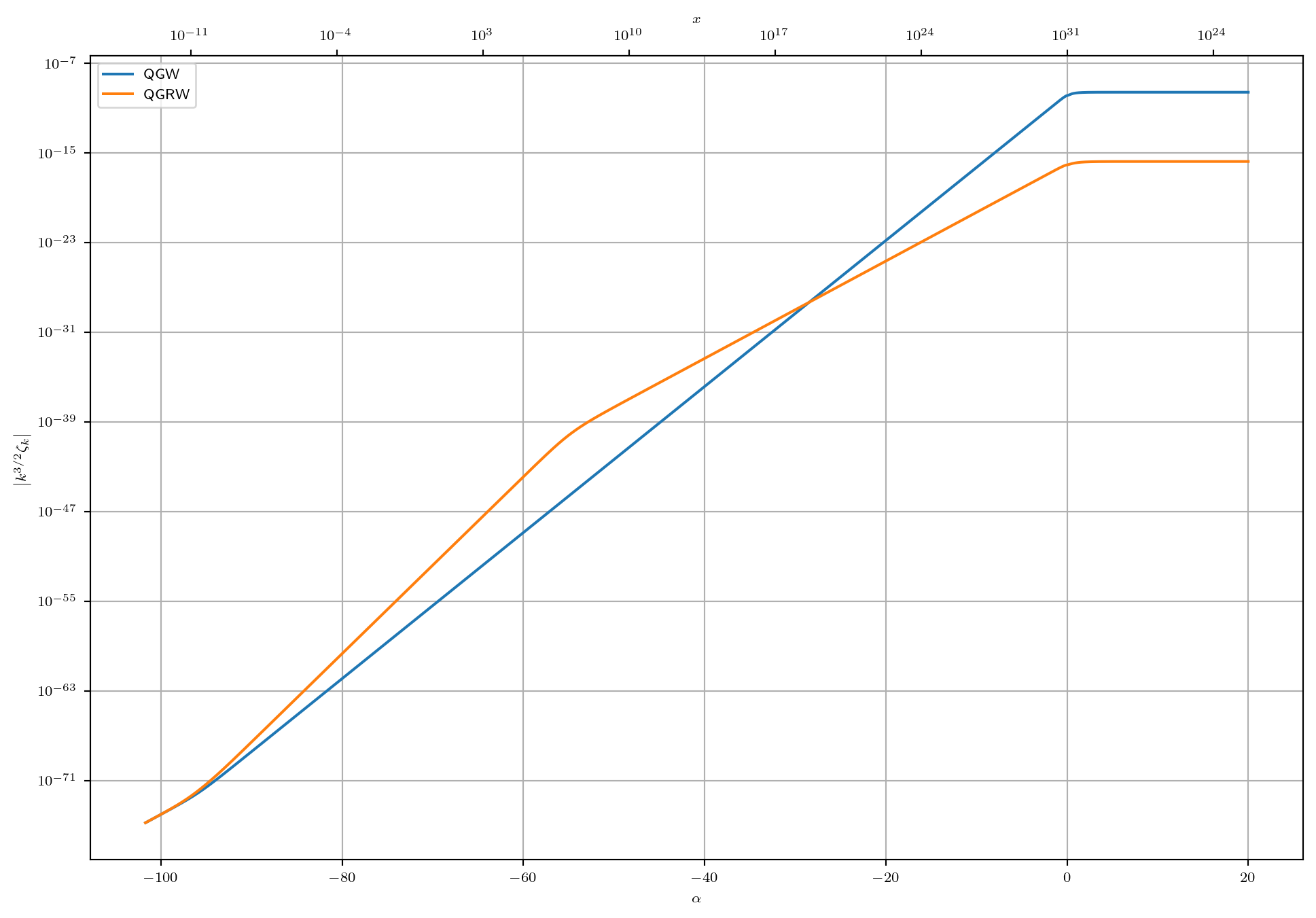
Both models yield the same result during the adiabatic regime and before radiation dominance. However, after radiation dominance, they diverge, with the QGRW model producing a smaller amplitude.
Mode \(k\) dependence
Before computing the actual power spectrum, we first check the \(k\) dependence of the mode. For that we plot the evolution of the mode for different \(k\) values.
Code
set_rc_params_article(ncol=1, nrows=1)
fig1, axs1 = plt.subplots()
fig2, axs2 = plt.subplots()

k_a = np.geomspace(1.0e-1 / RH_Mpc, 1.0e2, 10)
cmap = cm.viridis
norm = colors.LogNorm(vmin=min(k_a), vmax=max(k_a))
color_map = cm.ScalarMappable(cmap=cmap, norm=norm)
label_set = True

for k in k_a:
    adiab_w.set_k(RH_Mpc * k)
    adiab_rw.set_k(RH_Mpc * k)
    krh = RH_Mpc * k

    adiab_w.prepare(cosmo_w)
    tau_a, _ = adiab_w.get_time_array()
    field_sol_w = np.array(
        [
            np.array(adiab_w.eval_at(cosmo_w, tau, state).get_phi_Pphi()).flatten()
            for tau in tau_a
        ]
    )

    alpha_tau_a = np.array([alpha_of_tau(tau) for tau in tau_a])

    adiab_rw.prepare(cosmo_rw)
    alpha_a, _ = adiab_rw.get_time_array()
    field_sol_rw = np.array(
        [
            np.array(adiab_rw.eval_at(cosmo_rw, alpha, state).get_phi_Pphi()).flatten()
            for alpha in alpha_a
        ]
    )

    tau_alpha_a = np.array([tau_of_alpha(alpha) for alpha in alpha_a])

    axs1.plot(
        alpha_tau_a,
        unit_w * krh ** (1.5) * np.hypot(field_sol_w[:, 0], field_sol_w[:, 1]),
        color=cmap(norm(k)),
        linestyle="-",
        label=(
            f"QGW:$k={latex_float(k, convert_g=False)}\;[\mathrm{{Mpc}}^{{-1}}]$"
            if label_set
            else None
        ),
        lw=0.5,
    )
    axs2.plot(
        alpha_a,
        unit_rw * krh ** (1.5) * np.hypot(field_sol_rw[:, 0], field_sol_rw[:, 1]),
        color=cmap(norm(k)),
        linestyle="--",
        label=(
            f"QGRW:$k={latex_float(k, convert_g=False)}\;[\mathrm{{Mpc}}^{{-1}}]$"
            if label_set
            else None
        ),
        lw=0.5,
    )

    label_set = False

for ax in [axs1, axs2]:
    cbar = plt.colorbar(color_map, ax=ax, orientation="vertical")
    cbar.set_label(r"$k\;[\mathrm{Mpc}^{-1}]$")

    ax.set_yscale("log")
    ax.set_ylabel(r"$\left|k^{3/2}\zeta_k\right|$")
    ax.legend()
    ax.grid()

format_alpha_xaxis(axs1, cosmo_w)
format_alpha_xaxis(axs2, cosmo_rw)

fig1.savefig(f"{fig_dir}/adiabatic_k_dependence_w.pdf", bbox_inches="tight")
fig2.savefig(f"{fig_dir}/adiabatic_k_dependence_rw.pdf", bbox_inches="tight")

fig1.set_size_inches(6, 4)
fig2.set_size_inches(6, 4)

plt.show()
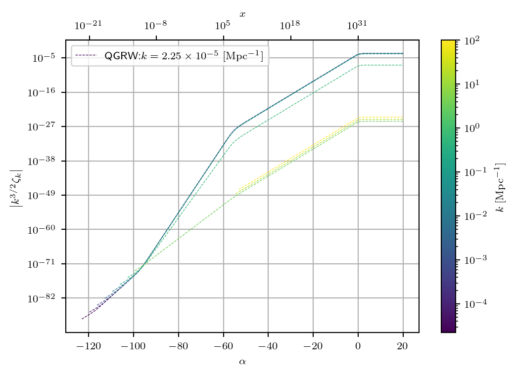
The QGW model, lacking a radiation component, exhibits an almost scale-invariant spectrum. In contrast, the QGRW model shows a \(k\)-dependence. In the QGRW model, smaller scales (larger \(k\)) are more influenced by the radiation component, introducing a \(k\)-dependence in the spectrum. Conversely, larger scales (smaller \(k\)) are dominated by the matter component, leading to an almost scale-invariant spectrum.
Power spectrum
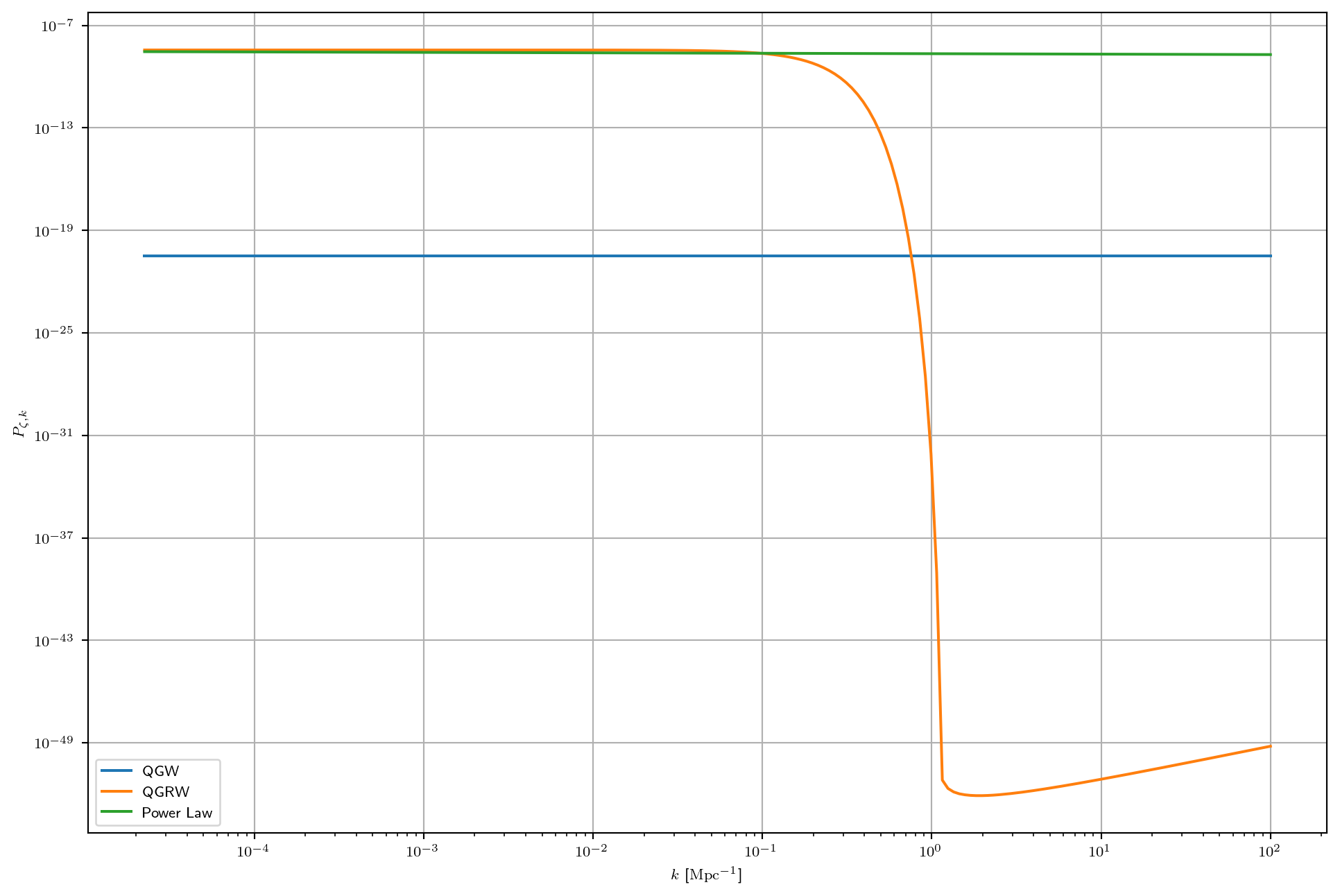
Now that we have checked the mode \(k\) dependence, we can compute the power spectrum. As a reference we also include the power spectrum of standard inflationary cosmology.
ps_k_a = np.geomspace(1.0e-1 / RH_Mpc, 1.0e2, 200)
tau_a = np.linspace(tau_end - 1.0, tau_end, 6)
alpha_a = np.linspace(alpha_end - 1.0, alpha_end, 6)

adiab_w.prepare_spectrum(cosmo_w, RH_Mpc * ps_k_a, tau_a)
Pzeta_w_spline = adiab_w.eval_powspec_zeta(cosmo_w)

Pzeta_w = np.array(
    [
        (RH_Mpc * k) ** 3 * Pzeta_w_spline.eval(cosmo_w, tau_end, RH_Mpc * k)
        for k in ps_k_a
    ]
)

adiab_rw.prepare_spectrum(cosmo_rw, RH_Mpc * ps_k_a, alpha_a)
Pzeta_rw_spline = adiab_rw.eval_powspec_zeta(cosmo_rw)
Pzeta_rw = np.array(
    [
        (RH_Mpc * k) ** 3 * Pzeta_rw_spline.eval(cosmo_rw, alpha_end, RH_Mpc * k)
        for k in ps_k_a
    ]
)

power_law = Nc.HIPrimPowerLaw.new()

Ppl = np.array([power_law.SA_powspec_k(k) for k in ps_k_a])
We plot the power spectrum for the QGW and QGRW models.
Code
set_rc_params_article(ncol=2, nrows=1)
fig, axs = plt.subplots()

axs.plot(ps_k_a, Pzeta_w, color="tab:blue", linestyle="-", label="QGW")
axs.plot(ps_k_a, Pzeta_rw, color="tab:orange", linestyle="-", label="QGRW")
axs.plot(ps_k_a, Ppl, color="tab:green", linestyle="-", label="Power Law")

axs.set_yscale("log")
axs.set_xscale("log")
axs.set_xlabel(r"$k$ [$\mathrm{Mpc}^{-1}$]")
axs.set_ylabel(r"$P_{\zeta,k}$")
axs.legend()
axs.grid()

plt.savefig(f"{fig_dir}/adiabatic_power_spectrum.pdf", bbox_inches="tight")

fig.set_size_inches(12, 8)

plt.show()