def doc_theme():
    return theme_minimal() + theme(
        panel_grid_minor=element_line(color="gray", linetype="--"),
)Recombination Evolution
Introduction
This example demonstrates the recombination evolution using the numcosmo library. We initialize the library, configure a cosmological model, and calculate the ionization history, equilibrium fractions, and visibility function.
Prerequisites
Before running this example, make sure the numcosmo_py1 package is installed in your environment. If it is not already installed, follow the installation instructions in the NumCosmo documentation. In addition, we are using numpy, matplotlib and pandas for data manipulation and plotting. If you are using the conda installation, these packages are already installed.
1 NumCosmo is a C library for cosmology and astrophysics that uses GObject-Introspection to provide bindings for various programming languages. To improve the user interface, we provide a Python package, numcosmo_py. This package imports all NumCosmo bindings and includes additional helper functions to simplify library usage.
Import and Initialize
First, import the required modules and initialize the NumCosmo library. We also import numpy, matplotlib and pandas. The Nc and Ncm modules provide the core functionality of the NumCosmo library. The call to Ncm.cfg_init() initializes the library objects.
import numpy as np
import pandas as pd
from plotnine import *

from numcosmo_py import Nc, Ncm

Ncm.cfg_init()
Recombination Evolution
The recombination evolution is calculated using the RecombSeager object. We set the precision to \(10^{-7}\) and the initial redshift to \(10^9\).
cosmo = Nc.HICosmoDEXcdm()
reion = Nc.HIReionCamb.new()
cosmo.add_submodel(reion)

recomb = Nc.RecombSeager(prec=1.0e-7, zi=1.0e9)

cosmo["H0"] = 70.0
cosmo["Omegac"] = 0.25
cosmo["Omegax"] = 0.70
cosmo["Tgamma0"] = 2.72
cosmo["Omegab"] = 0.05
cosmo["w"] = -1.00

recomb.prepare(cosmo)
We calculate the ionization history, equilibrium fractions, and visibility function.
alpha_a = np.log(np.geomspace(1.0e-4, 1.0e-2, 10000))
x_a = np.exp(-alpha_a)

# Compute ionization history and visibility function
ion_history = {
    "alpha": alpha_a,
    "x": np.exp(-alpha_a),
    "Xe": np.array([recomb.Xe(cosmo, alpha) for alpha in alpha_a]),
    "Xefi": np.array([recomb.equilibrium_Xe(cosmo, x) for x in x_a]),
    "XHI": np.array([recomb.equilibrium_XHI(cosmo, x) for x in x_a]),
    "XHII": np.array([recomb.equilibrium_XHII(cosmo, x) for x in x_a]),
    "XHeI": np.array([recomb.equilibrium_XHeI(cosmo, x) for x in x_a]),
    "XHeII": np.array([recomb.equilibrium_XHeII(cosmo, x) for x in x_a]),
    "XHeIII": np.array([recomb.equilibrium_XHeIII(cosmo, x) for x in x_a]),
    "v_tau": np.array([-recomb.v_tau(cosmo, alpha) for alpha in alpha_a]),
    "dv_tau_dlambda": np.array(
        [-recomb.dv_tau_dlambda(cosmo, alpha) / 10.0 for alpha in alpha_a]
    ),
    "d2v_tau_dlambda2": np.array(
        [-recomb.d2v_tau_dlambda2(cosmo, alpha) / 200.0 for alpha in alpha_a]
    ),
}
ion_history = pd.DataFrame(ion_history)

alpha_a = np.log(np.geomspace(1.0e-10, 1.0e-2, 10000))
x_a = np.exp(-alpha_a)

# Compute visibility function and derivatives
vis_func = {
    "alpha": alpha_a,
    "x": np.exp(-alpha_a),
    "dtau_dlambda": np.array([recomb.dtau_dlambda(cosmo, alpha) for alpha in alpha_a]),
    "x_E": np.array([x / np.sqrt(cosmo.E2(x)) for x in x_a]),
    "x_Etaub": np.array(
        [
            x / np.sqrt(cosmo.E2(x)) / abs(recomb.dtau_dlambda(cosmo, alpha))
            for alpha, x in zip(alpha_a, x_a)
        ]
    ),
}
vis_func = pd.DataFrame(vis_func)
Plot Ionization History
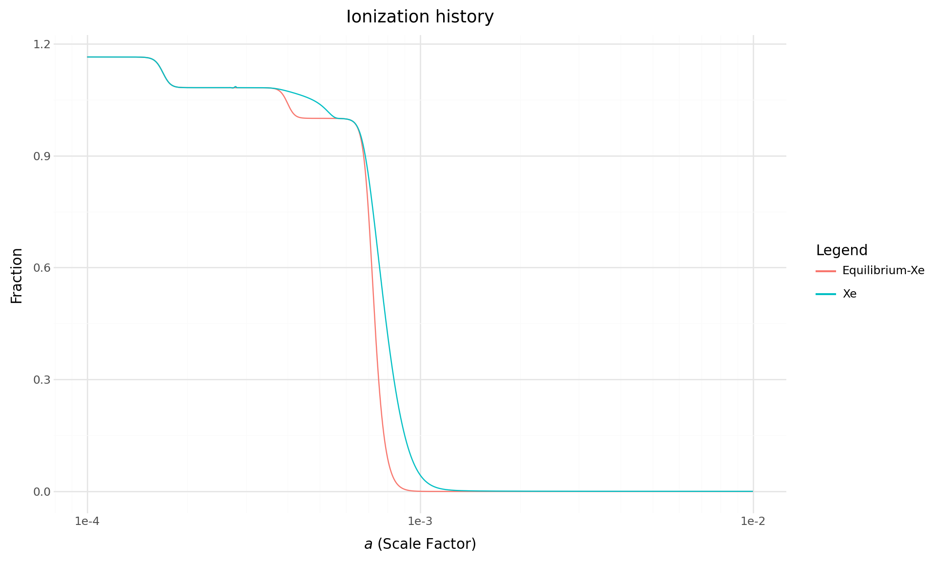
In the first plot, we compare the fraction of free electrons (\(X_e\)) with the equilibrium fraction of free electrons (\(X_{\text{efi}}\)) as functions of the scale factor.
- \(X_e\): Represents the actual ionization fraction of free electrons, determined by solving the Boltzmann equation, which accounts for the dynamical evolution of the ionization state.
- \(X_{\text{efi}}\): Represents the equilibrium fraction of free electrons, calculated assuming ionization equilibrium at each point in time.
This comparison highlights the deviation of \(X_e\) from \(X_{\text{efi}}\) due to the out-of-equilibrium processes that occur during recombination and reionization.
Code
ion_history_melted = ion_history.melt(
    id_vars="alpha",
    value_vars=["Xe", "Xefi"],
    var_name="Ion",
    value_name="Fraction",
)
ion_history_melted["Ion"] = ion_history_melted["Ion"].replace("Xefi", "Equilibrium-Xe")

(
    ggplot(ion_history_melted, aes(x="np.exp(alpha)", y="Fraction", color="Ion"))
    + geom_line()
    + labs(
        x=r"$a$ (Scale Factor)",
        y="Fraction",
        title="Ionization history",
        color="Legend",
    )
    + scale_x_log10()
    + theme_minimal()
    + theme(figure_size=(10, 6))
)
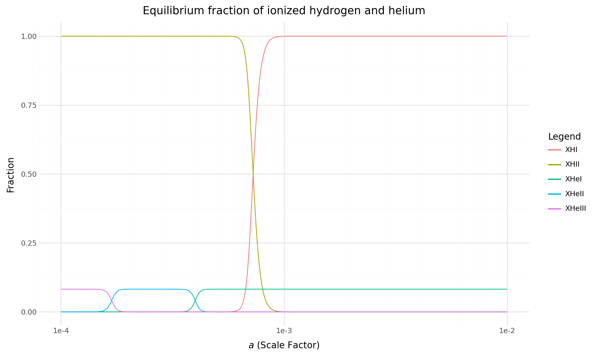
In a neutral cosmological model, the ionization fraction of free electrons, denoted as \(X_e\), is determined by the contributions from ionized hydrogen and helium. Specifically: \[X_e = X_{\text{HII}} + X_{\text{HeII}} + 2 X_{\text{HeIII}},\] where:
- \(X_{\text{HII}}\) represents the ionization fraction of ionized hydrogen.
- \(X_{\text{HeII}}\) is the ionization fraction of singly ionized helium.
- \(X_{\text{HeIII}}\) is the ionization fraction of doubly ionized helium (contributing twice due to the two free electrons per helium nucleus).
This relationship arises because each ionized hydrogen atom contributes one free electron, singly ionized helium contributes one free electron, and doubly ionized helium contributes two free electrons.
To better illustrate the contributions to the total ionization fraction, we also plot the individual ionization fractions \(X_{\text{HII}}\), \(X_{\text{HeII}}\), and \(X_{\text{HeIII}}\). This visualization highlights the relative contributions of hydrogen and helium ionization to the free electron fraction as the universe evolves.
Code
ion_history_melted = ion_history.melt(
    id_vars="alpha",
    value_vars=["XHI", "XHII", "XHeI", "XHeII", "XHeIII"],
    var_name="Ion",
    value_name="Fraction",
)

(
    ggplot(ion_history_melted, aes(x="np.exp(alpha)", y="Fraction", color="Ion"))
    + geom_line()
    + labs(
        x=r"$a$ (Scale Factor)",
        y="Fraction",
        title="Equilibrium fraction of ionized hydrogen and helium",
        color="Legend",
    )
    + scale_x_log10()
    + theme_minimal()
    + theme(figure_size=(10, 6))
)
Here’s the Quarto chunk that includes both the converted plotnine code and the accompanying description:
Visibility Function and Derivatives
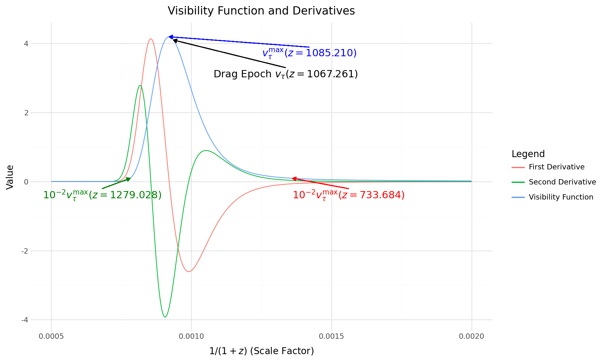
The following plot illustrates the visibility function \(v_\tau\) and its derivatives as functions of \(1+z\) on a logarithmic scale:
- \(v_\tau\): The visibility function, indicating the probability of photon decoupling at a given redshift.
- \(\frac{1}{10} \frac{dv_\tau}{d\lambda}\): The first derivative of \(v_\tau\), scaled by a factor of \(1/10\) for better visualization.
- \(\frac{1}{200} \frac{d^2v_\tau}{d\lambda^2}\): The second derivative of \(v_\tau\), scaled by a factor of \(1/200\).
The plot includes annotations highlighting key features: - The peak of the visibility function (\(v_\tau^{\text{max}}\)) and its corresponding redshift \(z\). - Points where \(v_\tau\) reaches \(10^{-2} \cdot v_\tau^{\text{max}}\), with their respective redshifts. - The redshift \(z^\star\), corresponding to the drag epoch (\(\tau = 1\)).
These features provide insight into the photon decoupling process and its dynamics during the recombination era.
Code
visibility_data = ion_history[
    (np.exp(ion_history["alpha"]) >= 0.0005) & (np.exp(ion_history["alpha"]) <= 0.002)
].melt(
    id_vars="alpha",
    value_vars=["v_tau", "dv_tau_dlambda", "d2v_tau_dlambda2"],
    var_name="Quantity",
    value_name="Value",
)

visibility_data["Quantity"] = visibility_data["Quantity"].replace(
    "v_tau", "Visibility Function"
)
visibility_data["Quantity"] = visibility_data["Quantity"].replace(
    "dv_tau_dlambda", "First Derivative"
)
visibility_data["Quantity"] = visibility_data["Quantity"].replace(
    "d2v_tau_dlambda2", "Second Derivative"
)

lambda_m, lambda_l, lambda_u = recomb.v_tau_lambda_features(cosmo, 2.0 * np.log(10.0))
v_tau_max = -recomb.v_tau(cosmo, lambda_m)
# lambda_l point where v_tau = 10^-2 * v_tau_max
v_tau_l = -recomb.v_tau(cosmo, lambda_l)
# lambda_u point where v_tau = 10^-2 * v_tau_max
v_tau_u = -recomb.v_tau(cosmo, lambda_u)

z_m = np.expm1(-lambda_m)
z_l = np.expm1(-lambda_l)
z_u = np.expm1(-lambda_u)

a_m = np.exp(lambda_m)
a_l = np.exp(lambda_l)
a_u = np.exp(lambda_u)

start_a_m = np.exp(lambda_m) + 5.0e-4
start_a_l = np.exp(lambda_l) - 1.0e-4
start_a_u = np.exp(lambda_u) + 2.0e-4

lambda_star = recomb.get_tau_drag_lambda(cosmo)
v_tau_star = -recomb.v_tau(cosmo, lambda_star)
z_star = np.expm1(-lambda_star)
a_star = np.exp(lambda_star)
start_a_star = np.exp(lambda_star) + 4.0e-4

(
    ggplot(visibility_data, aes(x="np.exp(alpha)", y="Value", color="Quantity"))
    + geom_line()
    + labs(
        x=r"$1/(1+z)$ (Scale Factor)",
        y="Value",
        title="Visibility Function and Derivatives",
        color="Legend",
    )
    + geom_segment(
        x=start_a_m,
        xend=a_m,
        y=v_tau_max - 0.3,
        yend=v_tau_max,
        color="blue",
        arrow=arrow(length=0.06, type="closed"),
    )
    + annotate(
        "text",
        x=start_a_m,
        y=v_tau_max - 0.5,
        label=rf"$v_\tau^{{\text{{max}}}} (z={z_m:.3f})$",
        color="blue",
        size=12,
    )
    + geom_segment(
        x=start_a_l,
        xend=a_l,
        y=v_tau_l - 0.3,
        yend=v_tau_l,
        color="green",
        arrow=arrow(length=0.06, type="closed"),
    )
    + annotate(
        "text",
        x=start_a_l,
        y=v_tau_l - 0.5,
        label=rf"$10^{{-2}} v_\tau^{{\text{{max}}}} (z={z_l:.3f})$",
        color="green",
        size=12,
    )
    + geom_segment(
        x=start_a_u,
        xend=a_u,
        y=v_tau_u - 0.3,
        yend=v_tau_u,
        color="red",
        arrow=arrow(length=0.06, type="closed"),
    )
    + annotate(
        "text",
        x=start_a_u,
        y=v_tau_u - 0.5,
        label=rf"$10^{{-2}} v_\tau^{{\text{{max}}}} (z={z_u:.3f})$",
        color="red",
        size=12,
    )
    + geom_segment(
        x=start_a_star,
        xend=a_star,
        y=v_tau_star - 0.8,
        yend=v_tau_star,
        color="black",
        arrow=arrow(length=0.06, type="closed"),
    )
    + annotate(
        "text",
        x=start_a_star,
        y=v_tau_star - 1.0,
        label=rf"Drag Epoch $v_\tau(z={z_star:.3f})$",
        color="black",
        size=12,
    )
    + theme_minimal()
    + theme(figure_size=(10, 6))
)
Optical Depth
We begin by calculating the optical depth as a function of redshift and scale factor.
alpha_a = np.log(np.geomspace(1.0e-10, 1.0e-2, 10000))
x_a = np.exp(-alpha_a)
dtau_dlambda_a = np.abs([recomb.dtau_dlambda(cosmo, alpha) for alpha in alpha_a])
E_a = np.array([cosmo.E(x) for x in x_a])
x_E_a = x_a / E_a
x_Etaub_a = x_E_a / dtau_dlambda_a

optical_depth = pd.DataFrame(
    {
        "alpha": alpha_a,
        "x": x_a,
        "dtau_dlambda": dtau_dlambda_a,
        "x_E": x_E_a,
        "x_Etaub": x_Etaub_a,
    }
)
In the code above, we compute the optical depth quantities: the differential optical depth (dtau_dlambda), x/E, and x/Etaub, based on the given redshift and scale factor.
Next, we plot the optical depth as a function of redshift and scale factor.
Code
optical_depth_melted = pd.melt(
    optical_depth,
    id_vars=["alpha", "x"],
    value_vars=["dtau_dlambda", "x_E", "x_Etaub"],
    var_name="Quantity",
    value_name="Value",
)

# Replacing the quantities' names for clarity
optical_depth_melted["Quantity"] = optical_depth_melted["Quantity"].replace(
    "dtau_dlambda", "Optical Depth"
)
optical_depth_melted["Quantity"] = optical_depth_melted["Quantity"].replace(
    "x_E", "x/E"
)
optical_depth_melted["Quantity"] = optical_depth_melted["Quantity"].replace(
    "x_Etaub", "x/Etaub"
)

# Plotting the optical depth
(
    ggplot(optical_depth_melted, aes(x="1/x", y="Value", color="Quantity"))
    + geom_line()
    + labs(
        x=r"$1/(1+z)$ (Scale Factor)",
        y="Value",
        title="Optical Depth",
        color="Legend",
    )
    + theme_minimal()
    + scale_x_log10()
    + scale_y_log10()
    + theme(figure_size=(10, 6))
)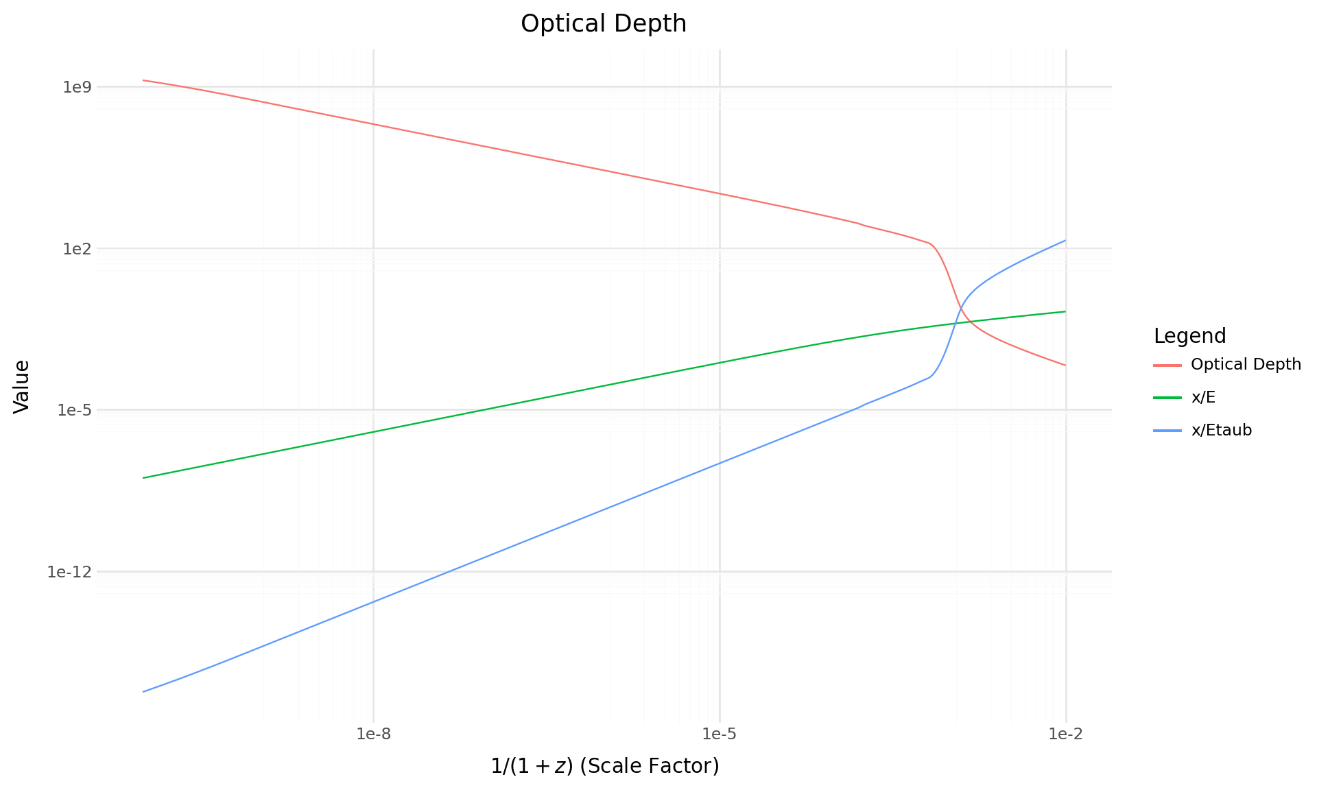
In this plot, we show the optical depth as a function of the scale factor \(1 + z\). We present the following quantities:
- Optical Depth: The differential optical depth (
dtau_dlambda). - \(\frac{x}{E}\): The ratio of the scale factor \(x\) to the energy \(E\).
- \(\frac{x}{\eta_{\tau}}\): The ratio of the scale factor \(x\) to the quantity \(\eta_{\tau}\).
We use a log-log scale for both axes to better visualize the changes across the broad range of values. The plot displays these quantities, making it easier to compare their behavior over the scale factor range.