import numpy as np
import pandas as pd
import matplotlib.pyplot as plt

from numcosmo_py import Nc, Ncm

Ncm.cfg_init()Dark Energy WSpline Background Evolution
Abstract
This example compares the dark-energy spline model NcHICosmoDEWSpline against the constant-\(w\) model NcHICosmoDEXcdm. It shows how to configure parameters using the dictionary-style API, assign knot values for the spline equation of state, and inspect the impact on background quantities and distances.
Introduction
This example compares two cosmologies with the same background parameters:
NcHICosmoDEXcdmwith constant \(w = -1\).NcHICosmoDEWSplinewith a knot-based \(w(z)\) history.
The notebook focuses on:
- dictionary-style parameter assignment (
cosmo["param"] = value), - spline-knot configuration using
w_iparameters, - a side-by-side comparison of \(w(z)\), background functions, and distances.
Import and Initialization
Build the Cosmological Models
We instantiate a 12-knot WSpline model and a reference XCDM model.
n_knots = 12
z_knots_max = 3.0

cosmo_ws = Nc.HICosmoDEWSpline.new(n_knots, z_knots_max)
cosmo_xcdm = Nc.HICosmoDEXcdm.new()
Set Parameters with the Dictionary API
The scalar cosmological parameters are assigned through dictionary-like access. This is the recommended high-level interface in Python examples.
base_params = {
    "H0": 70.0,
    "Omegac": 0.25,
    "Omegax": 0.70,
    "Omegab": 0.05,
    "Tgamma0": 2.72,
}

for key, value in base_params.items():
    cosmo_ws[key] = value
    cosmo_xcdm[key] = value

# Reference model: constant dark-energy equation of state.
cosmo_xcdm["w"] = -1.0
For the spline model, we assign one value per knot using the same dictionary-style API. The parameter names follow the w_i convention.
alpha_knots = np.array(cosmo_ws.get_alpha().dup_array())
z_knots = np.expm1(alpha_knots)

# Smooth toy profile: close to -1 at low/high z with a moderate excursion near z ~ 1.
w_knots = (
    -1.0
    + 0.18 * np.exp(-((z_knots - 0.9) / 0.55) ** 2)
    - 0.12 * np.exp(-((z_knots - 2.0) / 0.70) ** 2)
)

for i, w_i in enumerate(w_knots):
    cosmo_ws[f"w_{i}"] = float(w_i)
Prepare Background and Distance Calculators
dist = Nc.Distance.new(3.0)
dist.prepare(cosmo_ws)
Sample the Background Functions
z = np.linspace(0.0, 3.0, 240)

def evaluate_background(cosmo: Nc.HICosmo) -> pd.DataFrame:
    dist.prepare(cosmo)
    return pd.DataFrame(
        {
            "z": z,
            "w": [cosmo.w_de(zi) for zi in z],
            "E2": [cosmo.E2(zi) for zi in z],
            "E2Omega_de": [cosmo.E2Omega_de(zi) for zi in z],
            "dE2Omega_de_dz": [cosmo.dE2Omega_de_dz(zi) for zi in z],
            "d2E2Omega_de_dz2": [cosmo.d2E2Omega_de_dz2(zi) for zi in z],
            "Dc": [dist.comoving(cosmo, zi) for zi in z],
        }
    )

ws_df = evaluate_background(cosmo_ws)
xcdm_df = evaluate_background(cosmo_xcdm)

comparison = pd.DataFrame(
    {
        "z": z,
        "w_ws": ws_df["w"],
        "w_xcdm": xcdm_df["w"],
        "E2_rel_diff": ws_df["E2"] / xcdm_df["E2"] - 1.0,
        "E2Omega_de_rel_diff": ws_df["E2Omega_de"] / xcdm_df["E2Omega_de"] - 1.0,
        "Dc_rel_diff": ws_df["Dc"] / xcdm_df["Dc"] - 1.0,
    }
)

comparison.head(8)| z | w_ws | w_xcdm | E2_rel_diff | E2Omega_de_rel_diff | Dc_rel_diff | |
|---|---|---|---|---|---|---|
| 0 | 0.000000 | -0.987664 | -1.0 | 0.000000 | 0.000000 | NaN |
| 1 | 0.012552 | -0.986714 | -1.0 | 0.000332 | 0.000479 | -0.000082 |
| 2 | 0.025105 | -0.985708 | -1.0 | 0.000677 | 0.000989 | -0.000167 |
| 3 | 0.037657 | -0.984643 | -1.0 | 0.001035 | 0.001531 | -0.000253 |
| 4 | 0.050209 | -0.983515 | -1.0 | 0.001407 | 0.002106 | -0.000341 |
| 5 | 0.062762 | -0.982323 | -1.0 | 0.001793 | 0.002716 | -0.000432 |
| 6 | 0.075314 | -0.981063 | -1.0 | 0.002194 | 0.003363 | -0.000524 |
| 7 | 0.087866 | -0.979733 | -1.0 | 0.002608 | 0.004047 | -0.000619 |
Equation of State and Knot Placement
Code
fig, ax = plt.subplots(figsize=(9, 5))

ax.plot(z, ws_df["w"], lw=2.4, label="WSpline")
ax.plot(z, xcdm_df["w"], lw=1.8, ls="--", label="XCDM ($w=-1$)")
ax.scatter(z_knots, w_knots, s=30, zorder=3, label="WSpline knots")

ax.set_xlabel(r"$z$")
ax.set_ylabel(r"$w(z)$")
ax.set_title("Spline vs. Constant Dark-Energy Equation of State")
ax.grid(alpha=0.25)
ax.legend(loc="best")
plt.show()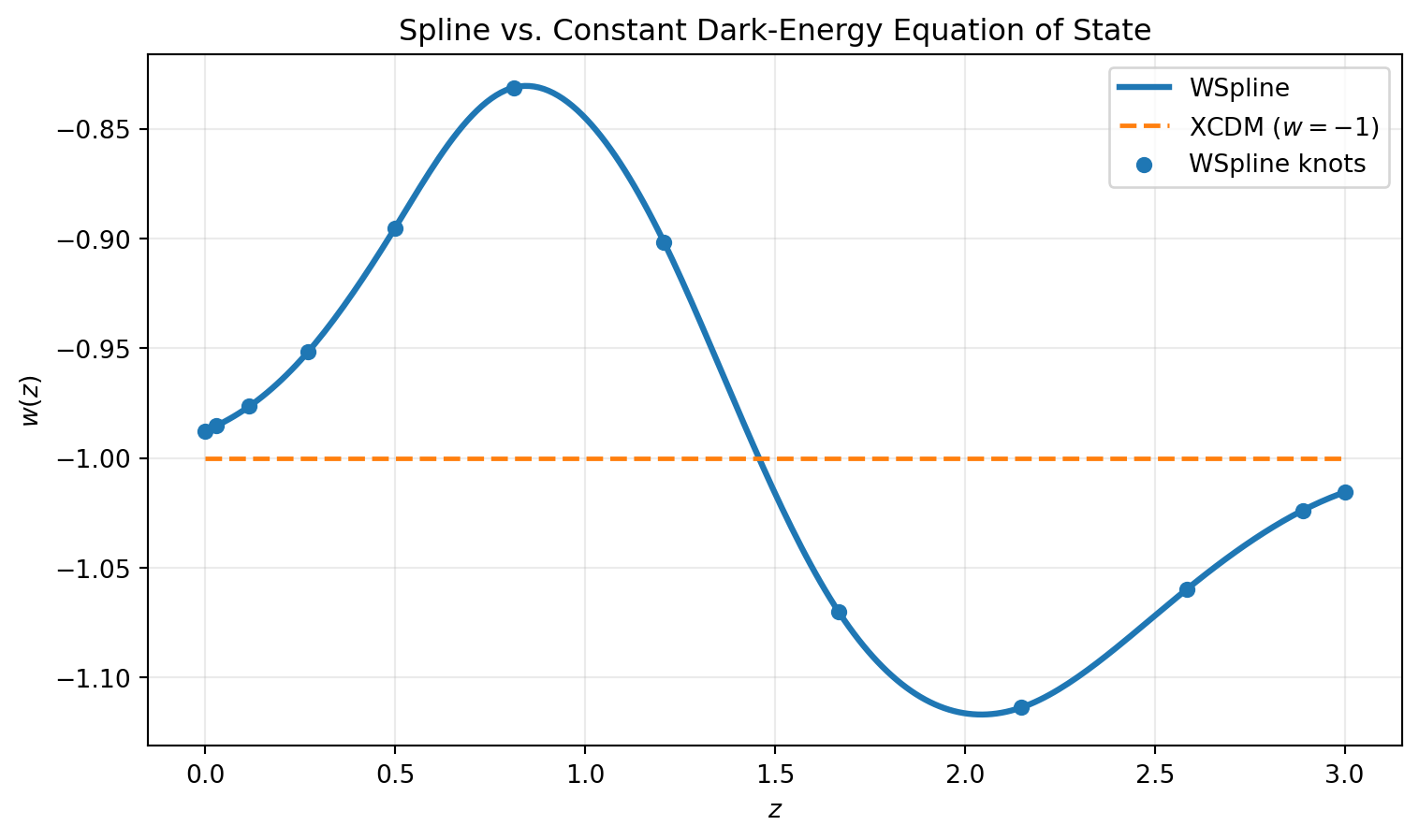
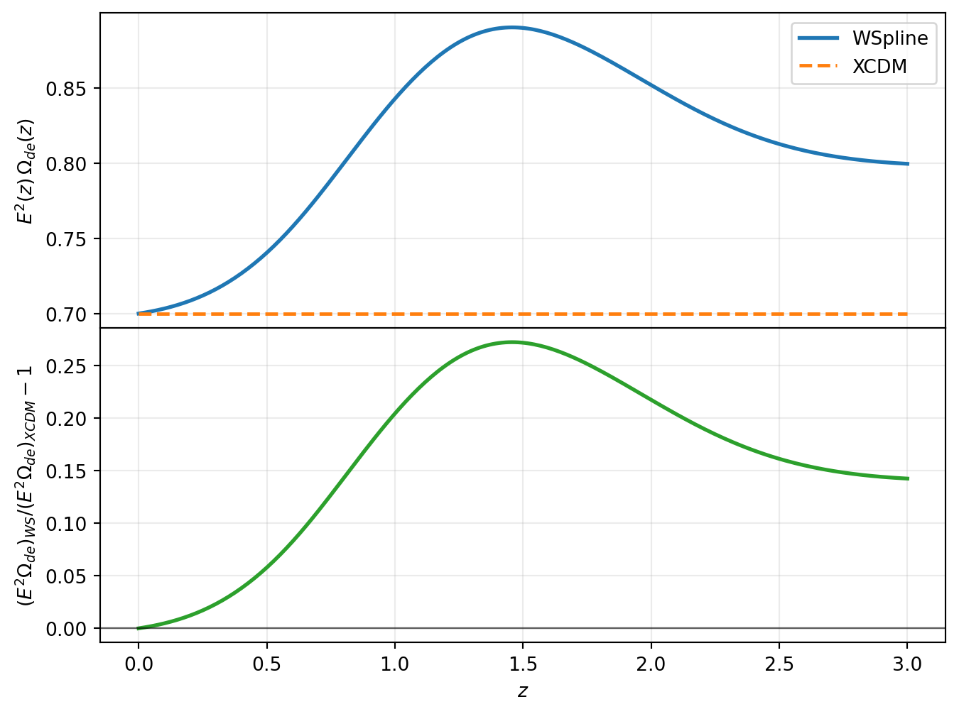
Background Functions
Code
fig1, axs1 = plt.subplots(2, 1, figsize=(8, 6), sharex=True)
fig1.subplots_adjust(hspace=0)

axs1[0].plot(z, ws_df["E2"], lw=2.0, label="WSpline")
axs1[0].plot(z, xcdm_df["E2"], lw=1.8, ls="--", label="XCDM")
axs1[0].set_ylabel(r"$E^2(z)$")
axs1[0].grid(alpha=0.25)
axs1[0].legend(loc="best")

axs1[1].plot(z, comparison["E2_rel_diff"], color="tab:red", lw=2.0)
axs1[1].axhline(0.0, color="black", lw=0.9, alpha=0.6)
axs1[1].set_xlabel(r"$z$")
axs1[1].set_ylabel(r"$E^2_{WS}/E^2_{XCDM} - 1$")
axs1[1].grid(alpha=0.25)

fig2, axs2 = plt.subplots(2, 1, figsize=(8, 6), sharex=True)
fig2.subplots_adjust(hspace=0)

axs2[0].plot(z, ws_df["E2Omega_de"], lw=2.0, label="WSpline")
axs2[0].plot(z, xcdm_df["E2Omega_de"], lw=1.8, ls="--", label="XCDM")
axs2[0].set_ylabel(r"$E^2(z)\,\Omega_{de}(z)$")
axs2[0].grid(alpha=0.25)
axs2[0].legend(loc="best")

axs2[1].plot(z, comparison["E2Omega_de_rel_diff"], color="tab:green", lw=2.0)
axs2[1].axhline(0.0, color="black", lw=0.9, alpha=0.6)
axs2[1].set_xlabel(r"$z$")
axs2[1].set_ylabel(r"$(E^2\Omega_{de})_{WS}/(E^2\Omega_{de})_{XCDM} - 1$")
axs2[1].grid(alpha=0.25)

plt.show()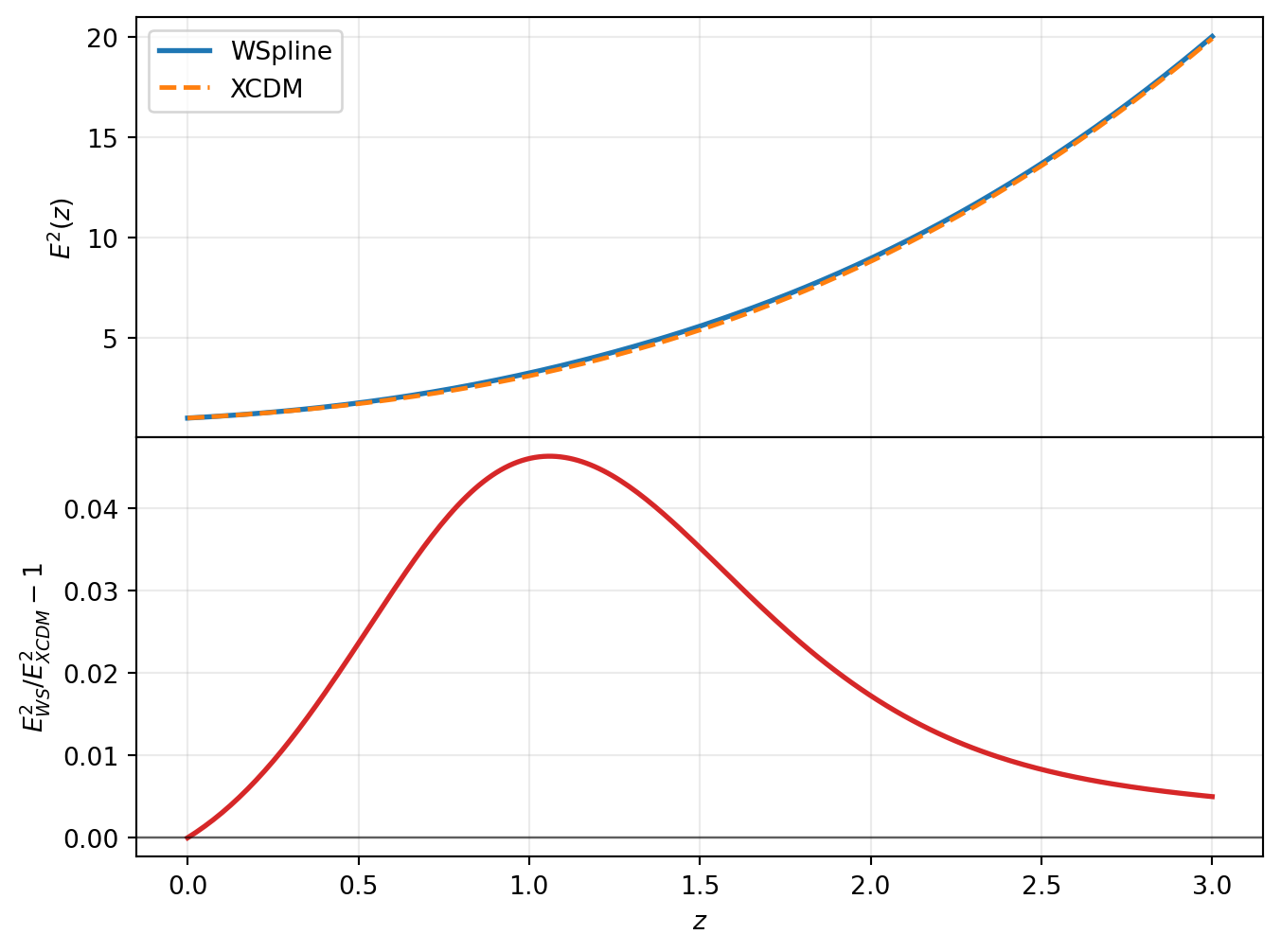
Dark-Energy Derivatives and Distance Effect
Code
fig1, axs1 = plt.subplots(2, 1, figsize=(8, 6), sharex=True)
fig1.subplots_adjust(hspace=0)
axs1[0].plot(z, ws_df["dE2Omega_de_dz"], lw=2.0, label="WSpline")
axs1[0].plot(z, xcdm_df["dE2Omega_de_dz"], lw=1.8, ls="--", label="XCDM")
axs1[0].set_ylabel(r"$d(E^2\Omega_{de})/dz$")
axs1[0].grid(alpha=0.25)
axs1[0].legend(loc="best")
axs1[1].plot(z, ws_df["d2E2Omega_de_dz2"], lw=2.0, label="WSpline")
axs1[1].plot(z, xcdm_df["d2E2Omega_de_dz2"], lw=1.8, ls="--", label="XCDM")
axs1[1].set_xlabel(r"$z$")
axs1[1].set_ylabel(r"$d^2(E^2\Omega_{de})/dz^2$")
axs1[1].grid(alpha=0.25)
fig2, ax2 = plt.subplots(figsize=(8, 6))
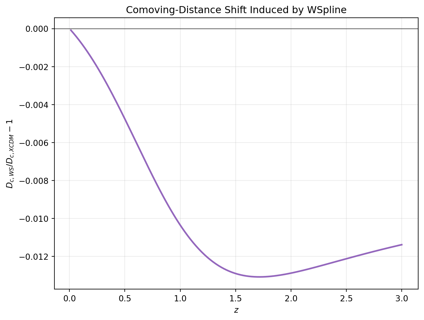
ax2.plot(z, comparison["Dc_rel_diff"], color="tab:purple", lw=2.0)
ax2.axhline(0.0, color="black", lw=0.9, alpha=0.6)
ax2.set_xlabel(r"$z$")
ax2.set_ylabel(r"$D_{c,WS}/D_{c,XCDM} - 1$")
ax2.set_title("Comoving-Distance Shift Induced by WSpline")
ax2.grid(alpha=0.25)
plt.show()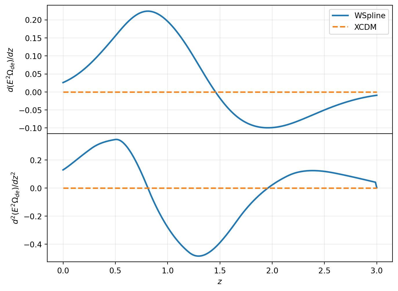
Conclusion
This example highlights WSpline background behavior with an emphasis on clear diagnostics. The parameter assignment uses:
- scalar parameters are set with dictionary access, and
- spline knot values are assigned with named entries (
w_0,w_1, …,w_{n-1}).
These comparisons provide a practical baseline for testing alternative \(w(z)\) knot configurations and quantifying their impact on background observables.