import sys
import numpy as np
import math
import matplotlib.pyplot as plt
from IPython.display import HTML, Markdown, display

# CCL
import pyccl
import pandas as pd

# NumCosmo
from numcosmo_py import Nc, Ncm
from numcosmo_py.ccl.nc_ccl import create_nc_obj, CCLParams, dsigmaM_dlnM

from numcosmo_py.plotting.tools import set_rc_params_article, format_time
import numcosmo_py.cosmology as ncc
import numcosmo_py.ccl.comparison as nc_cmpBenchmarking NumCosmo vs. CCL
Abstract
This document compares the two-point correlation implemented in NumCosmo and CCL.
Introduction
This notebook examines the two-point correlation functions and related quantities implemented in the Core Cosmology Library (CCL) and NumCosmo. Our goal is to evaluate the consistency and accuracy of these functions by analyzing their relative differences.
To this end, we define a set of cosmological models with fixed and variable parameters, then implement functions to compute and visualize the power spectra and their relative differences. The results are presented through tables and plots.
Initializing NumCosmo
To begin, we configure NumCosmo and redirect its output to this notebook using the following code:
Ncm.cfg_init()
Ncm.cfg_set_log_handler(lambda msg: sys.stdout.write(msg) and sys.stdout.flush())
set_rc_params_article(ncol=2, fontsize=12, use_tex=False)
Initial Parameter Definitions
We initialize the cosmological parameters and model-specific variables used for CCL and NumCosmo comparisons. Scalar parameters are fixed across all models, while arrays define variations in dark energy and neutrino properties for multiple scenarios. First, we instantiate a CCL cosmology object using the predefined global parameters. Next, using the numcosmo_py[^numcosmo_py] function create_nc_obj, we generate a NumCosmo cosmology object initialized with the same parameters as the CCL model. Fixed scalars apply universally, while arrays (\(\Omega_v\), \(w_0\), \(w_a\), \(m_\nu\)) represent different model configurations. Finally, in the setup_models function, one can enable high-precision computations in CCL, which increases accuracy at the cost of longer computation times. When this mode is activated, the overall agreement between CCL and NumCosmo improves significantly.
Code
from numcosmo_py.ccl.nc_ccl import create_nc_obj

PARAMETERS_SET = [
    r"$\Lambda$CDM, flat",
    r"$\Lambda$CDM, flat, $1\nu$",
    r"XCDM, flat",
    r"XCDM, spherical, $2\nu$",
    r"XCDM, hyperbolic",
]
COLORS = plt.rcParams["axes.prop_cycle"].by_key()["color"][:5]


def setup_models(
    Omega_c: float = 0.25,  # Cold dark matter density
    Omega_b: float = 0.05,  # Baryonic matter density
    h: float = 0.7,  # Dimensionless Hubble constant
    sigma8: float = 0.9,  # Matter density contrast std. dev. (8 Mpc/h)
    n_s: float = 0.96,  # Scalar spectral index
    Neff: float = 3.046,  # Effective number of massless neutrinos
    high_precision: bool = False,  # Use high precision computations in CCL
    dist_z_max: float = 15.0,  # Maximum redshift for distance computations
):
    """Setup cosmological models."""
    Omega_v_vals = np.array([0.7, 0.7, 0.7, 0.65, 0.75])  # Dark energy density
    w0_vals = np.array([-1.0, -1.0, -0.9, -0.9, -0.9])  # DE equation of state w0
    wa_vals = np.array([0.0, 0.0, 0.1, 0.1, 0.1])  # DE equation of state wa

    # Neutrino masses (eV) for each model: [m1, m2, m3]
    mnu = np.array(
        [
            [0.0, 0.0, 0.0],
            [0.04, 0.0, 0.0],
            [0.0, 0.0, 0.0],
            [0.03, 0.02, 0.0],
            [0.0, 0.0, 0.0],
        ]
    )
    Omega_k_vals = [
        float(1.0 - Omega_c - Omega_b - Omega_v) for Omega_v in Omega_v_vals
    ]

    parameters = [
        ["$\\Omega_c$", "Cold Dark Matter Density", Omega_c],
        ["$\\Omega_b$", "Baryonic Matter Density", Omega_b],
        ["$\\Omega_v$", "Dark Energy Density", Omega_v_vals],
        ["$\\Omega_k$", "Curvature Density", [f"{v:.3f}" for v in Omega_k_vals]],
        ["$h$", "Hubble Constant (dimensionless)", h],
        ["$n_s$", "Scalar Spectral Index", n_s],
        ["$N_\\mathrm{eff}$", "Effective Nº of Massless Neutrinos", Neff],
        ["$\\sigma_8$", "Matter Density Contrast Std. Dev. (8 Mpc/h)", sigma8],
        ["$w_0$", "DE Equation of State Parameter", w0_vals],
        ["$w_a$", "DE Equation of State Parameter", wa_vals],
        ["$m_\\nu$", "Neutrino Masses (eV)", [f"{m.tolist()}" for m in mnu]],
    ]
    models = []
    if high_precision:
        CCLParams.set_high_prec_params()

    for Omega_v, Omega_k, w0, wa, m in zip(
        Omega_v_vals, Omega_k_vals, w0_vals, wa_vals, mnu
    ):
        ccl_cosmo = pyccl.Cosmology(
            Omega_c=Omega_c,
            Omega_b=Omega_b,
            Neff=Neff,
            h=h,
            sigma8=sigma8,
            n_s=n_s,
            Omega_k=Omega_k,
            w0=w0,
            wa=wa,
            m_nu=m,
            transfer_function="eisenstein_hu",
        )
        cosmology = create_nc_obj(ccl_cosmo, dist_z_max=dist_z_max)
        models.append({"CCL": ccl_cosmo, "NC": cosmology})

    return parameters, models
# Preparing the models
parameters, models = setup_models(high_precision=False, dist_z_max=1500.0)
lmax = 3000
ells = np.arange(2, lmax + 1)
ell_kernel_test = 80Parameter Overview
The table below summarizes the parameter sets. We consider five sets, designed to cover a broad range of cosmologies, including models with and without neutrinos, spatial curvature, \(\Lambda\)CDM, and alternative values for the dark energy equation of state.
Code
# Create DataFrame
df = pd.DataFrame(parameters, columns=["Symbol", "Description", "Value"])
display(Markdown(df.to_markdown(index=False, colalign=["left"] * len(df.columns))))| Symbol | Description | Value |
|---|---|---|
| \(\Omega_c\) | Cold Dark Matter Density | 0.25 |
| \(\Omega_b\) | Baryonic Matter Density | 0.05 |
| \(\Omega_v\) | Dark Energy Density | [0.7 0.7 0.7 0.65 0.75] |
| \(\Omega_k\) | Curvature Density | [‘0.000’, ‘0.000’, ‘0.000’, ‘0.050’, ‘-0.050’] |
| \(h\) | Hubble Constant (dimensionless) | 0.7 |
| \(n_s\) | Scalar Spectral Index | 0.96 |
| \(N_\mathrm{eff}\) | Effective Nº of Massless Neutrinos | 3.046 |
| \(\sigma_8\) | Matter Density Contrast Std. Dev. (8 Mpc/h) | 0.9 |
| \(w_0\) | DE Equation of State Parameter | [-1. -1. -0.9 -0.9 -0.9] |
| \(w_a\) | DE Equation of State Parameter | [0. 0. 0.1 0.1 0.1] |
| \(m_\nu\) | Neutrino Masses (eV) | [‘[0.0, 0.0, 0.0]’, ‘[0.04, 0.0, 0.0]’, ‘[0.0, 0.0, 0.0]’, ‘[0.03, 0.02, 0.0]’, ‘[0.0, 0.0, 0.0]’] |
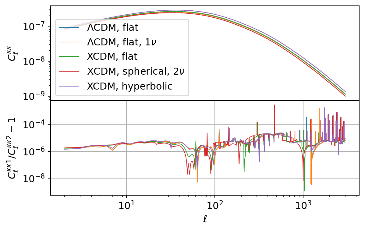
CMB Lensing
The following code compares the CMB lensing power spectrum implemented in CCL and NumCosmo. We plot the lensing kernel and power spectrum for each set.
cmb_len_auto_comparisons: list[nc_cmp.CompareFunc1d] = [
    [
        nc_cmp.compare_cmb_lens_kernel(m["CCL"], m["NC"], ell_kernel_test, model=name)
        for m, name in zip(models, PARAMETERS_SET)
    ],
    [
        nc_cmp.compare_cmb_len_auto(m["CCL"], m["NC"], ells, model=name)
        for m, name in zip(models, PARAMETERS_SET)
    ],
]
Code
for comparison in cmb_len_auto_comparisons:
    fig, axs = plt.subplots(2, sharex=True)
    fig.subplots_adjust(hspace=0)
    for p, c in zip(comparison, COLORS):
        p.plot(axs=axs, color=c)
    axs[1].grid()

    plt.show()
plt.close()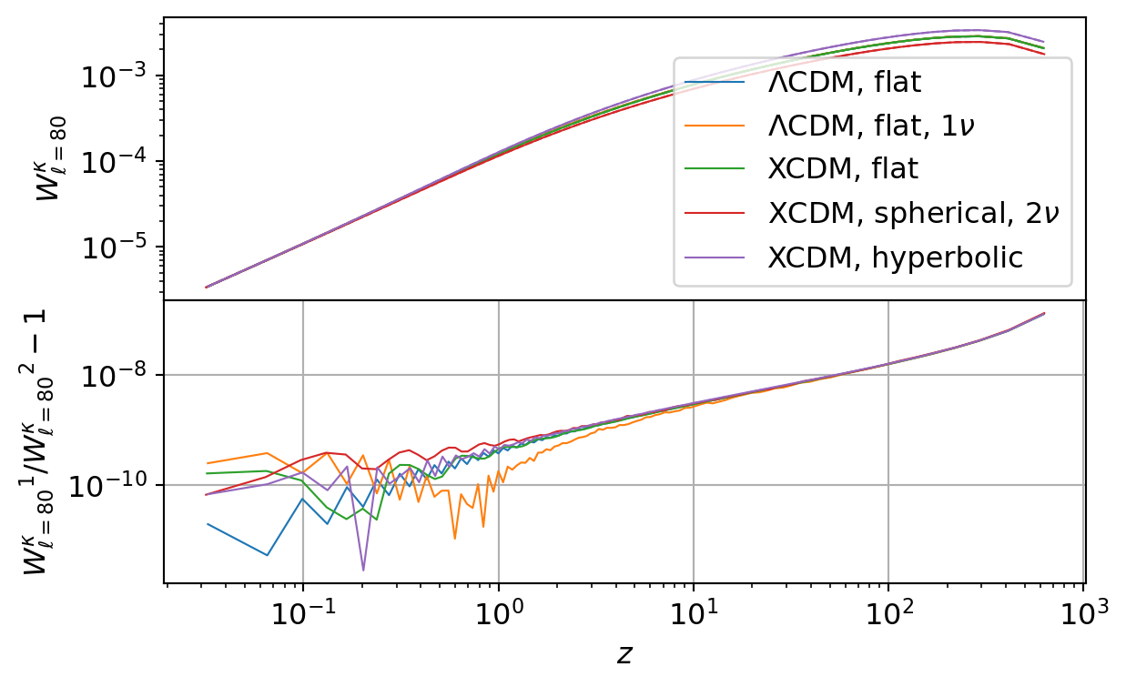
The following table summarizes the results for all sets.
Code
table = []

for comparison in cmb_len_auto_comparisons:
    for p in comparison:
        table.append(p.summary_row(convert_g=False))

df = pd.DataFrame(table, columns=nc_cmp.CompareFunc1d.table_header())
display(Markdown(df.to_markdown(index=False, colalign=["left"] * len(df.columns))))| Model | Quantity | \(\Delta P_{\text{min}}/P\) | \(\Delta P_{\text{max}}/P\) | \(\overline{\Delta P / P}\) | \(\sigma_{\Delta P / P}\) |
|---|---|---|---|---|---|
| \(\Lambda\)CDM, flat | \({W_{\ell={80}}^\kappa}\) | \(5.25 \times 10^{-12}\) | \(1.27 \times 10^{-7}\) | \(5.48 \times 10^{-9}\) | \(1.51 \times 10^{-8}\) |
| \(\Lambda\)CDM, flat, \(1\nu\) | \({W_{\ell={80}}^\kappa}\) | \(1.06 \times 10^{-11}\) | \(1.28 \times 10^{-7}\) | \(5.29 \times 10^{-9}\) | \(1.53 \times 10^{-8}\) |
| XCDM, flat | \({W_{\ell={80}}^\kappa}\) | \(2.34 \times 10^{-11}\) | \(1.29 \times 10^{-7}\) | \(5.56 \times 10^{-9}\) | \(1.53 \times 10^{-8}\) |
| XCDM, spherical, \(2\nu\) | \({W_{\ell={80}}^\kappa}\) | \(6.65 \times 10^{-11}\) | \(1.33 \times 10^{-7}\) | \(5.81 \times 10^{-9}\) | \(1.59 \times 10^{-8}\) |
| XCDM, hyperbolic | \({W_{\ell={80}}^\kappa}\) | \(2.80 \times 10^{-12}\) | \(1.27 \times 10^{-7}\) | \(5.61 \times 10^{-9}\) | \(1.52 \times 10^{-8}\) |
| \(\Lambda\)CDM, flat | \({C_\ell^{\kappa\kappa}}\) | \(6.11 \times 10^{-8}\) | \(1.53 \times 10^{-3}\) | \(8.40 \times 10^{-6}\) | \(3.79 \times 10^{-5}\) |
| \(\Lambda\)CDM, flat, \(1\nu\) | \({C_\ell^{\kappa\kappa}}\) | \(3.26 \times 10^{-9}\) | \(1.71 \times 10^{-3}\) | \(9.31 \times 10^{-6}\) | \(4.98 \times 10^{-5}\) |
| XCDM, flat | \({C_\ell^{\kappa\kappa}}\) | \(1.17 \times 10^{-9}\) | \(7.71 \times 10^{-4}\) | \(8.33 \times 10^{-6}\) | \(2.72 \times 10^{-5}\) |
| XCDM, spherical, \(2\nu\) | \({C_\ell^{\kappa\kappa}}\) | \(6.40 \times 10^{-9}\) | \(2.82 \times 10^{-3}\) | \(9.39 \times 10^{-6}\) | \(5.78 \times 10^{-5}\) |
| XCDM, hyperbolic | \({C_\ell^{\kappa\kappa}}\) | \(5.58 \times 10^{-8}\) | \(1.73 \times 10^{-3}\) | \(8.75 \times 10^{-6}\) | \(3.95 \times 10^{-5}\) |
All CCL calculations are consistent with the results from NumCosmo, though this agreement decreases as the number of samples increases.
This counterintuitive behavior occurs because CCL computes the distance from \(z_\mathrm{lss}\) to \(z\) as the difference between their comoving distances, rather than directly calculating the distance between the two redshifts. As the number of samples increases, \(\chi(z_\mathrm{lss})\) and \(\chi(z)\) become more similar, leading to a cancellation error that dominates the kernel.
Additionally, several spikes appear in the relative difference of \(C_\ell^{\kappa\kappa}\), which are attributed to errors in the CCL Limber integration.
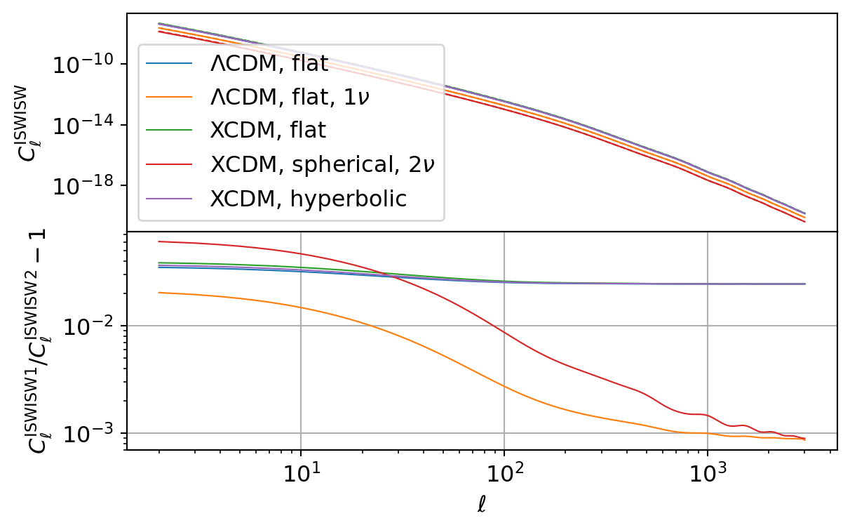
CMB Integrated Sachs-Wolfe (ISW)
The following code compares the CMB ISW power spectrum as implemented in CCL and NumCosmo. We show both the ISW kernel and the final \(C_\ell\) values to highlight the agreement and differences between the two frameworks.
cmb_isw_auto_comparisons: list[nc_cmp.CompareFunc1d] = [
    [
        nc_cmp.compare_cmb_isw_kernel(m["CCL"], m["NC"], ell_kernel_test, model=name)
        for m, name in zip(models, PARAMETERS_SET)
    ],
    [
        nc_cmp.compare_cmb_isw_auto(m["CCL"], m["NC"], ells, model=name)
        for m, name in zip(models, PARAMETERS_SET)
    ],
]
Code
for comparison in cmb_isw_auto_comparisons:
    fig, axs = plt.subplots(2, sharex=True)
    fig.subplots_adjust(hspace=0)
    for p, c in zip(comparison, COLORS):
        p.plot(axs=axs, color=c)
    axs[1].grid()

    plt.show()
plt.close()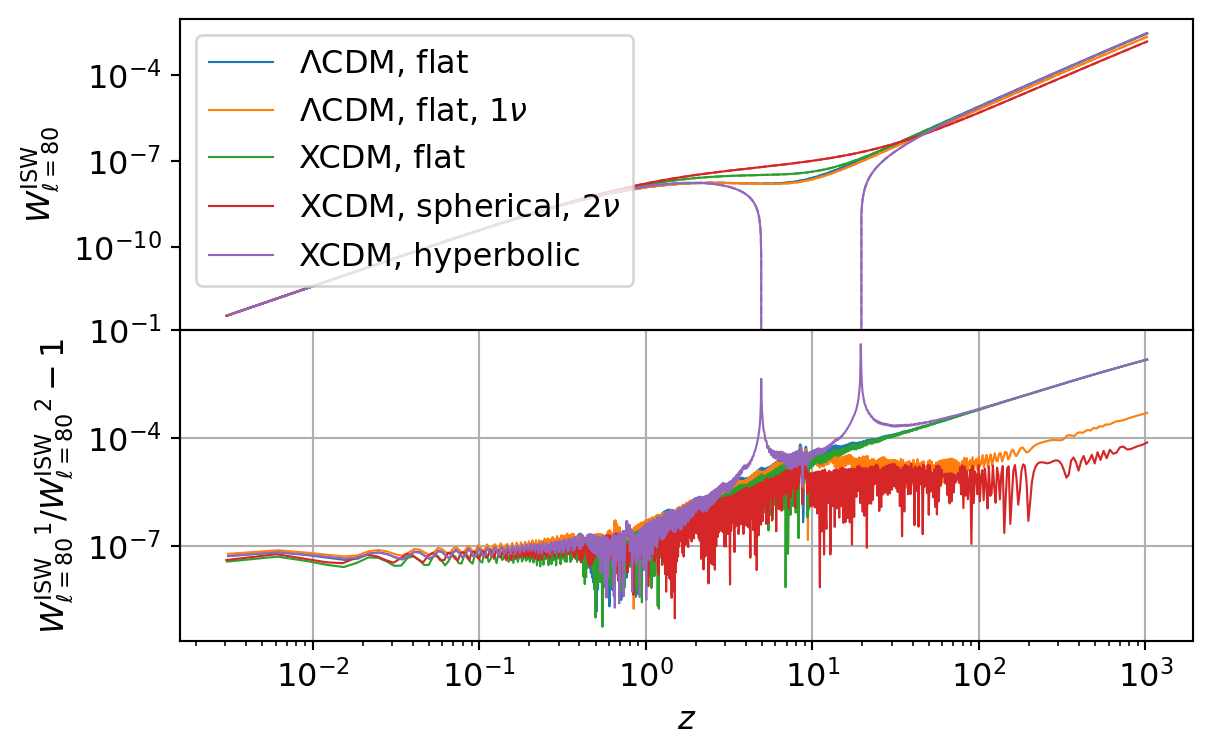
The following table summarizes the results for all sets.
Code
table = []

for comparison in cmb_isw_auto_comparisons:
    for p in comparison:
        table.append(p.summary_row(convert_g=False))

df = pd.DataFrame(table, columns=nc_cmp.CompareFunc1d.table_header())
display(Markdown(df.to_markdown(index=False, colalign=["left"] * len(df.columns))))| Model | Quantity | \(\Delta P_{\text{min}}/P\) | \(\Delta P_{\text{max}}/P\) | \(\overline{\Delta P / P}\) | \(\sigma_{\Delta P / P}\) |
|---|---|---|---|---|---|
| \(\Lambda\)CDM, flat | \({W_{\ell={80}}^\mathrm{ISW}}\) | \(1.53 \times 10^{-9}\) | \(1.56 \times 10^{-2}\) | \(3.13 \times 10^{-4}\) | \(1.38 \times 10^{-3}\) |
| \(\Lambda\)CDM, flat, \(1\nu\) | \({W_{\ell={80}}^\mathrm{ISW}}\) | \(1.80 \times 10^{-9}\) | \(5.09 \times 10^{-4}\) | \(1.65 \times 10^{-5}\) | \(4.39 \times 10^{-5}\) |
| XCDM, flat | \({W_{\ell={80}}^\mathrm{ISW}}\) | \(5.69 \times 10^{-10}\) | \(1.56 \times 10^{-2}\) | \(3.13 \times 10^{-4}\) | \(1.39 \times 10^{-3}\) |
| XCDM, spherical, \(2\nu\) | \({W_{\ell={80}}^\mathrm{ISW}}\) | \(9.84 \times 10^{-10}\) | \(7.67 \times 10^{-5}\) | \(4.67 \times 10^{-6}\) | \(8.18 \times 10^{-6}\) |
| XCDM, hyperbolic | \({W_{\ell={80}}^\mathrm{ISW}}\) | \(1.93 \times 10^{-9}\) | \(4.18 \times 10^{-2}\) | \(4.18 \times 10^{-4}\) | \(1.92 \times 10^{-3}\) |
| \(\Lambda\)CDM, flat | \({C_\ell^{\mathrm{ISW}\mathrm{ISW}}}\) | \(2.43 \times 10^{-2}\) | \(3.48 \times 10^{-2}\) | \(2.45 \times 10^{-2}\) | \(7.10 \times 10^{-4}\) |
| \(\Lambda\)CDM, flat, \(1\nu\) | \({C_\ell^{\mathrm{ISW}\mathrm{ISW}}}\) | \(8.65 \times 10^{-4}\) | \(2.03 \times 10^{-2}\) | \(1.21 \times 10^{-3}\) | \(1.34 \times 10^{-3}\) |
| XCDM, flat | \({C_\ell^{\mathrm{ISW}\mathrm{ISW}}}\) | \(2.44 \times 10^{-2}\) | \(3.84 \times 10^{-2}\) | \(2.47 \times 10^{-2}\) | \(1.02 \times 10^{-3}\) |
| XCDM, spherical, \(2\nu\) | \({C_\ell^{\mathrm{ISW}\mathrm{ISW}}}\) | \(8.95 \times 10^{-4}\) | \(6.05 \times 10^{-2}\) | \(2.23 \times 10^{-3}\) | \(4.62 \times 10^{-3}\) |
| XCDM, hyperbolic | \({C_\ell^{\mathrm{ISW}\mathrm{ISW}}}\) | \(2.44 \times 10^{-2}\) | \(3.64 \times 10^{-2}\) | \(2.46 \times 10^{-2}\) | \(8.20 \times 10^{-4}\) |
The CCL calculations show marginal agreement with those from NumCosmo. This discrepancy stems from CCL’s reduced accuracy in computing the growth function and growth factor at high redshifts (\(z \gtrsim 10\)). While this limitation does not significantly impact cross-correlations involving the ISW kernel when combined with probes anchored at lower redshifts, it introduces pronounced errors in the ISW autocorrelation, which depends on precise integration over the full redshift range up to \(\z_\mathrm{lss}\).
As illustrated in the ISW kernel plot, the results exhibit strong agreement up to \(z \sim 10\), beyond which discrepancies grow increasingly pronounced, reflecting the cumulative effect of inaccuracies in CCL’s high-\(z\) growth calculations.
Thermal Sunyaev-Zel’dovich (tSZ) Effect
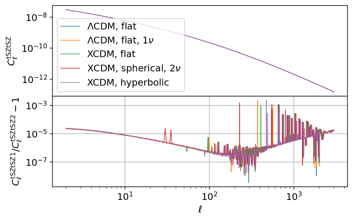
The code below benchmarks the thermal Sunyaev-Zel’dovich (tSZ) kernel and angular power spectrum (\(C_\ell\)) implementations in CCL and NumCosmo. This comparison cross-validates the two frameworks, focusing on relative differences in the kernel and \(C_\ell\) values.
tsz_auto_comparisons: list[nc_cmp.CompareFunc1d] = [
    [
        nc_cmp.compare_tsz_kernel(m["CCL"], m["NC"], ell_kernel_test, model=name)
        for m, name in zip(models, PARAMETERS_SET)
    ],
    [
        nc_cmp.compare_tsz_auto(m["CCL"], m["NC"], ells, model=name)
        for m, name in zip(models, PARAMETERS_SET)
    ],
]
Code
for comparison in tsz_auto_comparisons:
    fig, axs = plt.subplots(2, sharex=True)
    fig.subplots_adjust(hspace=0)
    for p, c in zip(comparison, COLORS):
        p.plot(axs=axs, color=c)
    axs[1].grid()

    plt.show()
plt.close()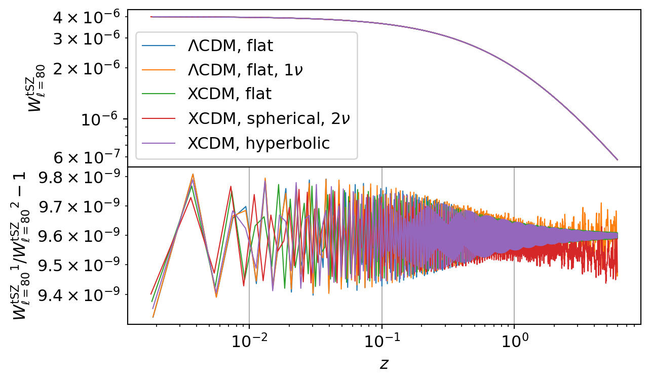
The following table summarizes the results for all sets.
Code
table = []

for comparison in tsz_auto_comparisons:
    for p in comparison:
        table.append(p.summary_row(convert_g=False))

df = pd.DataFrame(table, columns=nc_cmp.CompareFunc1d.table_header())
display(Markdown(df.to_markdown(index=False, colalign=["left"] * len(df.columns))))| Model | Quantity | \(\Delta P_{\text{min}}/P\) | \(\Delta P_{\text{max}}/P\) | \(\overline{\Delta P / P}\) | \(\sigma_{\Delta P / P}\) |
|---|---|---|---|---|---|
| \(\Lambda\)CDM, flat | \({W_{\ell={80}}^\mathrm{tSZ}}\) | \(9.33 \times 10^{-9}\) | \(9.81 \times 10^{-9}\) | \(9.60 \times 10^{-9}\) | \(5.40 \times 10^{-11}\) |
| \(\Lambda\)CDM, flat, \(1\nu\) | \({W_{\ell={80}}^\mathrm{tSZ}}\) | \(9.33 \times 10^{-9}\) | \(9.81 \times 10^{-9}\) | \(9.60 \times 10^{-9}\) | \(5.97 \times 10^{-11}\) |
| XCDM, flat | \({W_{\ell={80}}^\mathrm{tSZ}}\) | \(9.38 \times 10^{-9}\) | \(9.77 \times 10^{-9}\) | \(9.60 \times 10^{-9}\) | \(4.96 \times 10^{-11}\) |
| XCDM, spherical, \(2\nu\) | \({W_{\ell={80}}^\mathrm{tSZ}}\) | \(9.40 \times 10^{-9}\) | \(9.77 \times 10^{-9}\) | \(9.56 \times 10^{-9}\) | \(5.62 \times 10^{-11}\) |
| XCDM, hyperbolic | \({W_{\ell={80}}^\mathrm{tSZ}}\) | \(9.35 \times 10^{-9}\) | \(9.79 \times 10^{-9}\) | \(9.60 \times 10^{-9}\) | \(5.12 \times 10^{-11}\) |
| \(\Lambda\)CDM, flat | \({C_\ell^{\mathrm{tSZ}\mathrm{tSZ}}}\) | \(3.45 \times 10^{-9}\) | \(1.15 \times 10^{-3}\) | \(1.05 \times 10^{-5}\) | \(3.42 \times 10^{-5}\) |
| \(\Lambda\)CDM, flat, \(1\nu\) | \({C_\ell^{\mathrm{tSZ}\mathrm{tSZ}}}\) | \(1.77 \times 10^{-8}\) | \(2.36 \times 10^{-3}\) | \(1.18 \times 10^{-5}\) | \(5.88 \times 10^{-5}\) |
| XCDM, flat | \({C_\ell^{\mathrm{tSZ}\mathrm{tSZ}}}\) | \(7.86 \times 10^{-9}\) | \(1.16 \times 10^{-3}\) | \(1.08 \times 10^{-5}\) | \(3.86 \times 10^{-5}\) |
| XCDM, spherical, \(2\nu\) | \({C_\ell^{\mathrm{tSZ}\mathrm{tSZ}}}\) | \(1.37 \times 10^{-8}\) | \(1.60 \times 10^{-3}\) | \(1.16 \times 10^{-5}\) | \(5.03 \times 10^{-5}\) |
| XCDM, hyperbolic | \({C_\ell^{\mathrm{tSZ}\mathrm{tSZ}}}\) | \(1.02 \times 10^{-8}\) | \(2.32 \times 10^{-3}\) | \(1.16 \times 10^{-5}\) | \(5.51 \times 10^{-5}\) |
All CCL calculations show good agreement with the results from NumCosmo.
However, the same Limber integration errors present in CCL also manifest here, leading to eventual spikes in the relative difference between the two frameworks at random multipoles (\(\ell\)).
Galaxy Weak Lensing
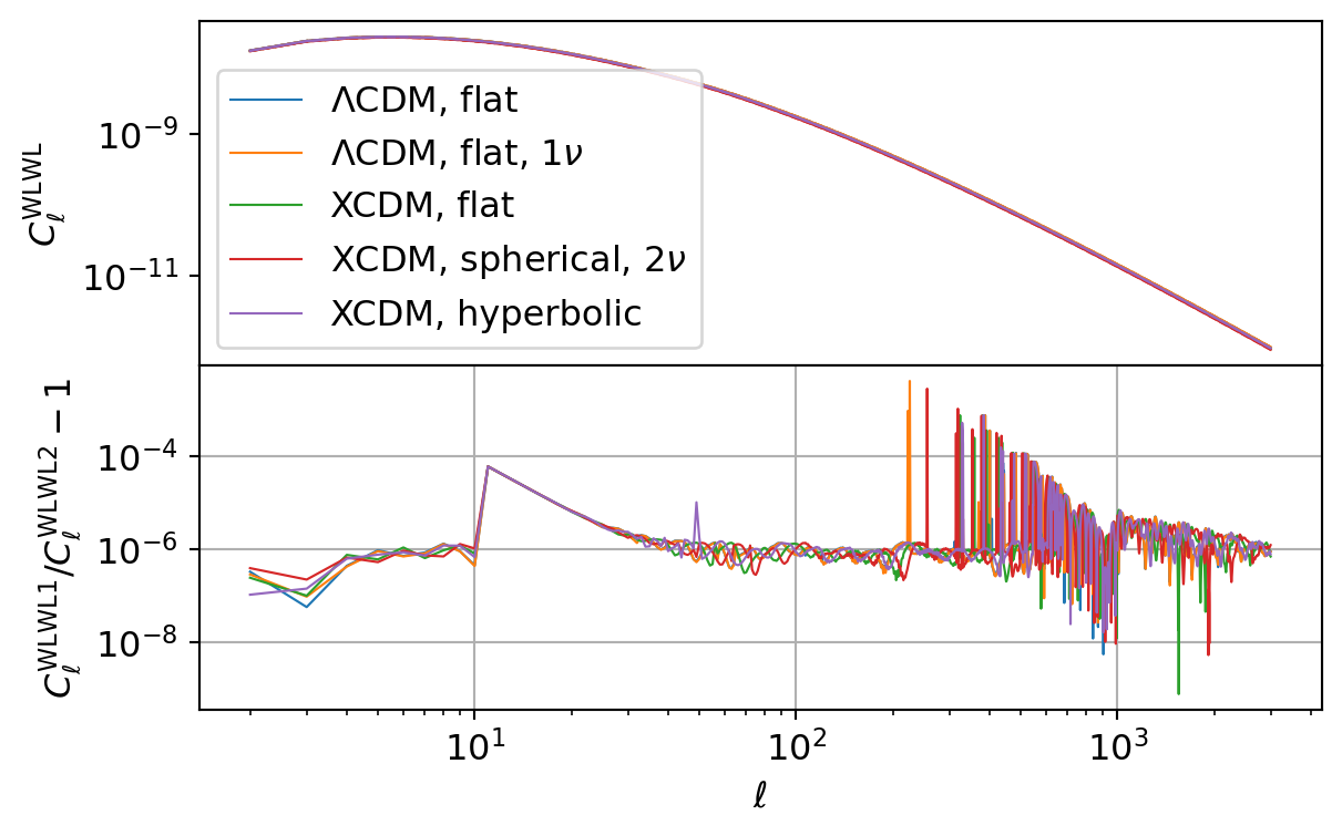
The following code compares the galaxy weak lensing kernel and angular power spectrum implemented in CCL and NumCosmo.
gwl_auto_comparisons: list[nc_cmp.CompareFunc1d] = [
    [
        nc_cmp.compare_galaxy_weak_lensing_kernel(
            m["CCL"], m["NC"], ell_kernel_test, model=name
        )
        for m, name in zip(models, PARAMETERS_SET)
    ],
    [
        nc_cmp.compare_galaxy_weak_lensing_auto(m["CCL"], m["NC"], ells, model=name)
        for m, name in zip(models, PARAMETERS_SET)
    ],
]
Code
for comparison in gwl_auto_comparisons:
    fig, axs = plt.subplots(2, sharex=True)
    fig.subplots_adjust(hspace=0)
    for p, c in zip(comparison, COLORS):
        p.plot(axs=axs, color=c)
    axs[1].grid()

    plt.show()
plt.close()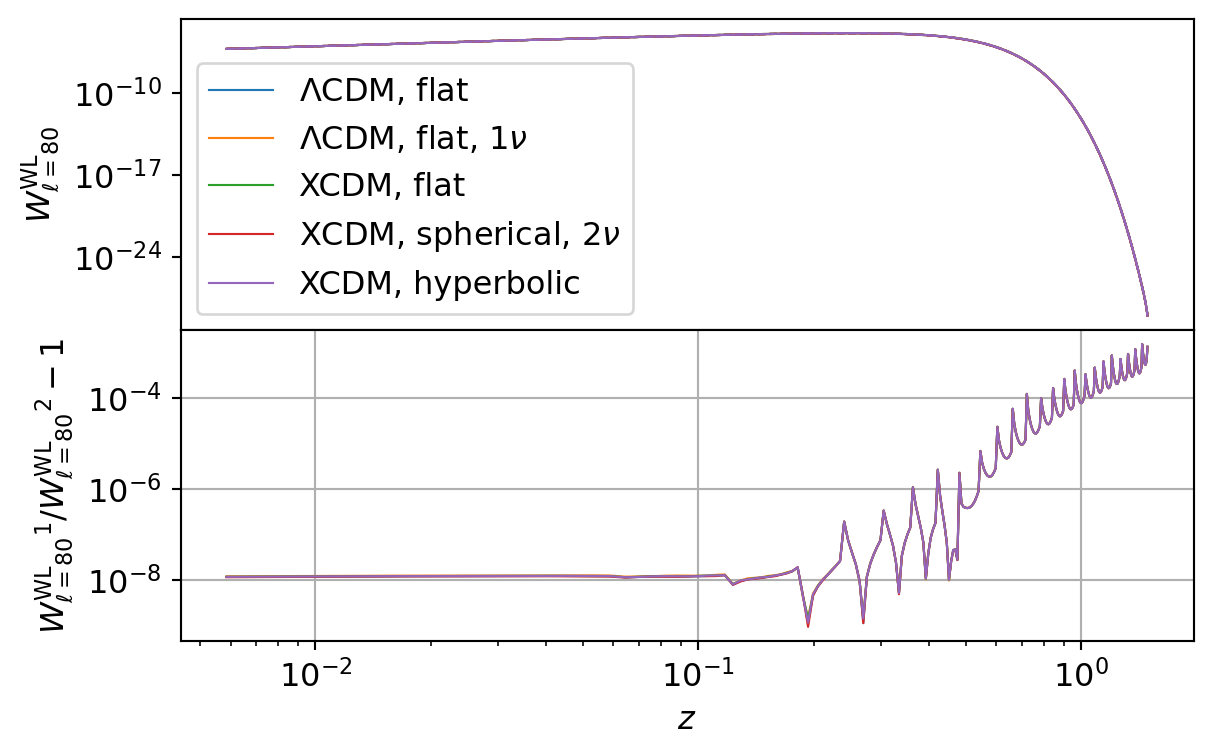
The following table summarizes the results for all sets.
Code
table = []

for comparison in gwl_auto_comparisons:
    for p in comparison:
        table.append(p.summary_row(convert_g=False))

df = pd.DataFrame(table, columns=nc_cmp.CompareFunc1d.table_header())
display(Markdown(df.to_markdown(index=False, colalign=["left"] * len(df.columns))))| Model | Quantity | \(\Delta P_{\text{min}}/P\) | \(\Delta P_{\text{max}}/P\) | \(\overline{\Delta P / P}\) | \(\sigma_{\Delta P / P}\) |
|---|---|---|---|---|---|
| \(\Lambda\)CDM, flat | \({W_{\ell={80}}^\mathrm{WL}}\) | \(1.09 \times 10^{-9}\) | \(1.59 \times 10^{-3}\) | \(1.45 \times 10^{-4}\) | \(2.46 \times 10^{-4}\) |
| \(\Lambda\)CDM, flat, \(1\nu\) | \({W_{\ell={80}}^\mathrm{WL}}\) | \(1.44 \times 10^{-9}\) | \(1.59 \times 10^{-3}\) | \(1.45 \times 10^{-4}\) | \(2.46 \times 10^{-4}\) |
| XCDM, flat | \({W_{\ell={80}}^\mathrm{WL}}\) | \(1.35 \times 10^{-9}\) | \(1.59 \times 10^{-3}\) | \(1.45 \times 10^{-4}\) | \(2.46 \times 10^{-4}\) |
| XCDM, spherical, \(2\nu\) | \({W_{\ell={80}}^\mathrm{WL}}\) | \(9.05 \times 10^{-10}\) | \(1.59 \times 10^{-3}\) | \(1.45 \times 10^{-4}\) | \(2.46 \times 10^{-4}\) |
| XCDM, hyperbolic | \({W_{\ell={80}}^\mathrm{WL}}\) | \(1.13 \times 10^{-9}\) | \(1.59 \times 10^{-3}\) | \(1.45 \times 10^{-4}\) | \(2.46 \times 10^{-4}\) |
| \(\Lambda\)CDM, flat | \({C_\ell^{\mathrm{WL}\mathrm{WL}}}\) | \(5.60 \times 10^{-9}\) | \(7.38 \times 10^{-4}\) | \(3.19 \times 10^{-6}\) | \(1.68 \times 10^{-5}\) |
| \(\Lambda\)CDM, flat, \(1\nu\) | \({C_\ell^{\mathrm{WL}\mathrm{WL}}}\) | \(2.67 \times 10^{-8}\) | \(4.00 \times 10^{-3}\) | \(4.79 \times 10^{-6}\) | \(7.67 \times 10^{-5}\) |
| XCDM, flat | \({C_\ell^{\mathrm{WL}\mathrm{WL}}}\) | \(7.87 \times 10^{-10}\) | \(7.37 \times 10^{-4}\) | \(3.76 \times 10^{-6}\) | \(2.34 \times 10^{-5}\) |
| XCDM, spherical, \(2\nu\) | \({C_\ell^{\mathrm{WL}\mathrm{WL}}}\) | \(5.40 \times 10^{-9}\) | \(2.74 \times 10^{-3}\) | \(4.89 \times 10^{-6}\) | \(5.75 \times 10^{-5}\) |
| XCDM, hyperbolic | \({C_\ell^{\mathrm{WL}\mathrm{WL}}}\) | \(1.65 \times 10^{-8}\) | \(7.42 \times 10^{-4}\) | \(3.62 \times 10^{-6}\) | \(2.01 \times 10^{-5}\) |
All CCL calculations agree with the results from NumCosmo. Again the same Limber integration errors present in CCL also manifest here, leading to eventual spikes in the relative difference between the two frameworks at random multipoles (\(\ell\)).
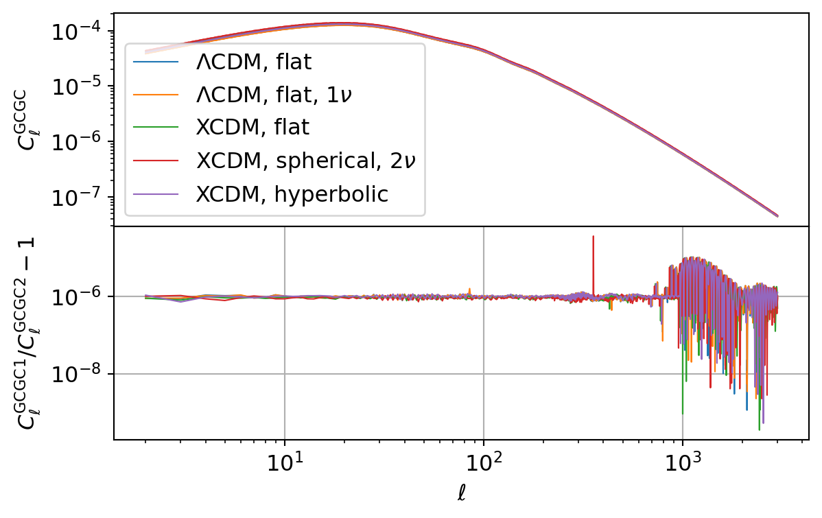
Galaxy Number Count
The following code compares the galaxy number count power spectrum implemented in CCL and NumCosmo.
gnc_auto_comparisons: list[nc_cmp.CompareFunc1d] = [
    [
        nc_cmp.compare_galaxy_number_count_kernel(
            m["CCL"], m["NC"], ell_kernel_test, model=name
        )
        for m, name in zip(models, PARAMETERS_SET)
    ],
    [
        nc_cmp.compare_galaxy_number_count_auto(m["CCL"], m["NC"], ells, model=name)
        for m, name in zip(models, PARAMETERS_SET)
    ]
]
Code
for comparison in gnc_auto_comparisons:
    fig, axs = plt.subplots(2, sharex=True)
    fig.subplots_adjust(hspace=0)
    for p, c in zip(comparison, COLORS):
        p.plot(axs=axs, color=c)
    axs[1].grid()

    plt.show()
plt.close()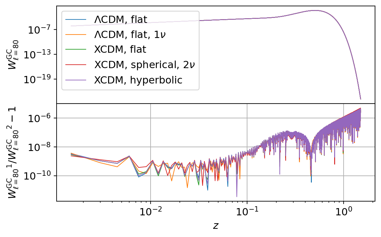
The following table summarizes the results for all sets.
Code
table = []

for comparison in gnc_auto_comparisons:
    for p in comparison:
        table.append(p.summary_row(convert_g=False))

df = pd.DataFrame(table, columns=nc_cmp.CompareFunc1d.table_header())
display(Markdown(df.to_markdown(index=False, colalign=["left"] * len(df.columns))))| Model | Quantity | \(\Delta P_{\text{min}}/P\) | \(\Delta P_{\text{max}}/P\) | \(\overline{\Delta P / P}\) | \(\sigma_{\Delta P / P}\) |
|---|---|---|---|---|---|
| \(\Lambda\)CDM, flat | \({W_{\ell={80}}^\mathrm{GC}}\) | \(9.74 \times 10^{-12}\) | \(4.20 \times 10^{-6}\) | \(6.15 \times 10^{-7}\) | \(8.70 \times 10^{-7}\) |
| \(\Lambda\)CDM, flat, \(1\nu\) | \({W_{\ell={80}}^\mathrm{GC}}\) | \(1.45 \times 10^{-11}\) | \(4.21 \times 10^{-6}\) | \(6.14 \times 10^{-7}\) | \(8.70 \times 10^{-7}\) |
| XCDM, flat | \({W_{\ell={80}}^\mathrm{GC}}\) | \(2.24 \times 10^{-11}\) | \(4.80 \times 10^{-6}\) | \(7.08 \times 10^{-7}\) | \(1.01 \times 10^{-6}\) |
| XCDM, spherical, \(2\nu\) | \({W_{\ell={80}}^\mathrm{GC}}\) | \(2.05 \times 10^{-11}\) | \(5.03 \times 10^{-6}\) | \(7.36 \times 10^{-7}\) | \(1.06 \times 10^{-6}\) |
| XCDM, hyperbolic | \({W_{\ell={80}}^\mathrm{GC}}\) | \(3.41 \times 10^{-12}\) | \(4.53 \times 10^{-6}\) | \(6.78 \times 10^{-7}\) | \(9.54 \times 10^{-7}\) |
| \(\Lambda\)CDM, flat | \({C_{\ell}^{\mathrm{GC}\mathrm{GC}}}\) | \(1.13 \times 10^{-9}\) | \(1.05 \times 10^{-5}\) | \(1.82 \times 10^{-6}\) | \(2.00 \times 10^{-6}\) |
| \(\Lambda\)CDM, flat, \(1\nu\) | \({C_{\ell}^{\mathrm{GC}\mathrm{GC}}}\) | \(2.25 \times 10^{-9}\) | \(1.05 \times 10^{-5}\) | \(1.83 \times 10^{-6}\) | \(2.00 \times 10^{-6}\) |
| XCDM, flat | \({C_{\ell}^{\mathrm{GC}\mathrm{GC}}}\) | \(3.44 \times 10^{-10}\) | \(1.05 \times 10^{-5}\) | \(1.78 \times 10^{-6}\) | \(2.00 \times 10^{-6}\) |
| XCDM, spherical, \(2\nu\) | \({C_{\ell}^{\mathrm{GC}\mathrm{GC}}}\) | \(2.23 \times 10^{-9}\) | \(3.68 \times 10^{-5}\) | \(1.69 \times 10^{-6}\) | \(2.00 \times 10^{-6}\) |
| XCDM, hyperbolic | \({C_{\ell}^{\mathrm{GC}\mathrm{GC}}}\) | \(5.15 \times 10^{-10}\) | \(1.05 \times 10^{-5}\) | \(1.84 \times 10^{-6}\) | \(2.01 \times 10^{-6}\) |
The results are in very good agreement with the results from NumCosmo. Note the same Limber integration errors present in CCL also manifest here.
Time Comparison
The following code compares the time measurements between CCL and NumCosmo.
# Lets first get a simple dndz function. We use 1000 knots and a width of 0.1.
dndz = nc_cmp.prepare_dndz(0.5, 0.1, 1000)
z_a = np.array(dndz.peek_xv().dup_array())
nz_a = np.array(dndz.peek_yv().dup_array())
nc_wl_auto_v = Ncm.Vector.new(lmax + 1 - 2)
bias = 3.0
mbias = 1.234


def compute_wl_using_ccl(
    ccl_cosmo: pyccl.Cosmology, z_a: np.ndarray, nz_a: np.ndarray, ells: np.ndarray
):
    ccl_wl = pyccl.WeakLensingTracer(ccl_cosmo, dndz=(z_a, nz_a))
    psp = ccl_cosmo.get_linear_power()
    ccl_wl_auto = pyccl.angular_cl(
        ccl_cosmo, ccl_wl, ccl_wl, ells, p_of_k_a_lin=psp, p_of_k_a=psp
    )

    return ccl_wl_auto


def compute_nc_using_ccl(
    ccl_cosmo: pyccl.Cosmology,
    z_a: np.ndarray,
    nz_a: np.ndarray,
    ells: np.ndarray,
    bias: float,
    mbias: float,
) -> np.ndarray:
    ccl_gal = pyccl.NumberCountsTracer(
        ccl_cosmo,
        has_rsd=False,
        dndz=(z_a, nz_a),
        bias=(z_a, np.ones_like(z_a) * bias),
        mag_bias=(z_a, np.ones_like(z_a) * mbias),
    )

    psp = ccl_cosmo.get_linear_power()
    ccl_gal_auto = pyccl.angular_cl(
        ccl_cosmo, ccl_gal, ccl_gal, ells, p_of_k_a_lin=psp, p_of_k_a=psp
    )

    return ccl_gal_auto


def compute_wl_using_nc(
    cosmology: ncc.Cosmology,
    dndz: Ncm.Spline,
    ells: np.ndarray,
    nc_wl_auto_v: Ncm.Vector,
):
    nc_wl = Nc.XcorKernelWeakLensing.new(
        cosmology.dist, cosmology.ps_ml, dndz, 3.0, 7.0
    )
    xcor = Nc.Xcor.new(cosmology.dist, cosmology.ps_ml, Nc.XcorMethod.LIMBER_Z_CUBATURE)
    xcor.prepare(cosmology.cosmo)
    nc_wl.prepare(cosmology.cosmo)
    xcor.compute(nc_wl, nc_wl, cosmology.cosmo, 2, lmax, nc_wl_auto_v)

    return np.array(nc_wl_auto_v.dup_array())


def compute_nc_using_nc(
    cosmology: ncc.Cosmology,
    dndz: Ncm.Spline,
    ells: np.ndarray,
    bias: float,
    mbias: float,
    nc_wl_auto_v: Ncm.Vector,
) -> np.ndarray:
    nc_gal = Nc.XcorKernelGal.new(cosmology.dist, cosmology.ps_ml, 1, 3.0, dndz, True)
    nc_gal["mag_bias"] = mbias
    nc_gal["bparam_0"] = bias
    xcor = Nc.Xcor.new(cosmology.dist, cosmology.ps_ml, Nc.XcorMethod.LIMBER_Z_CUBATURE)
    nc_gal.prepare(cosmology.cosmo)
    xcor.prepare(cosmology.cosmo)
    xcor.compute(nc_gal, nc_gal, cosmology.cosmo, 2, lmax, nc_wl_auto_v)

    return np.array(nc_wl_auto_v.dup_array())


table = [
    ["Galaxy Weak Lensing", "CCL"]
    + nc_cmp.compute_times(
        lambda: compute_wl_using_ccl(models[0]["CCL"], z_a, nz_a, ells),
        repeat=5,
        number=10,
    ),
    ["Galaxy Weak Lensing", "NumCosmo"]
    + nc_cmp.compute_times(
        lambda: compute_wl_using_nc(models[0]["NC"], dndz, ells, nc_wl_auto_v),
        repeat=5,
        number=10,
    ),
    ["Galaxy Number Counts", "CCL"]
    + nc_cmp.compute_times(
        lambda: compute_nc_using_ccl(models[1]["CCL"], z_a, nz_a, ells, bias, mbias),
        repeat=5,
        number=10,
    ),
    ["Galaxy Number Counts", "NumCosmo"]
    + nc_cmp.compute_times(
        lambda: compute_nc_using_nc(
            models[1]["NC"], dndz, ells, bias, mbias, nc_wl_auto_v
        ),
        repeat=5,
        number=10,
    ),
]

columns = ["Quantity", "Library", "Mean Time", "Standard Deviation"]

df = pd.DataFrame(table, columns=columns)
df["Mean Time"] = df["Mean Time"].apply(format_time)
df["Standard Deviation"] = df["Standard Deviation"].apply(format_time)

display(Markdown(df.to_markdown(index=False, colalign=["left"] * len(df.columns))))| Quantity | Library | Mean Time | Standard Deviation |
|---|---|---|---|
| Galaxy Weak Lensing | CCL | 39.34 ms | 46.17 \(\mu\)s |
| Galaxy Weak Lensing | NumCosmo | 74.87 ms | 1.82 ms |
| Galaxy Number Counts | CCL | 103.82 ms | 392.37 \(\mu\)s |
| Galaxy Number Counts | NumCosmo | 104.88 ms | 2.22 ms |
Summary
In summary, the two frameworks demonstrate strong agreement across most calculations, with discrepancies at random multipoles (\(\ell\)). These differences are due to the Limber integral errors in CCL, which introduces numerical inaccuracies whenever the integration fails. Additionally, the ISW computation in CCL exhibits large deviations at high redshifts (\(z \gtrsim 10\)), stemming from inaccuracies in the growth function and growth factor. While these errors do not significantly impact cross-correlations with low-redshift probes, they become critical in the ISW autocorrelation, which depends on precise integration over the full redshift range up to \(z_\mathrm{lss}\).
The Limber integration errors in CCL further manifest as spikes in random values of \(\ell\), particularly, when there is good agreement between the two frameworks they become more noticeable.