def doc_theme():
    return theme_minimal() + theme(
        panel_grid_minor=element_line(color="gray", linetype="--"),
)Computing Bounce Spectra
Purpose
This tutorial shows how to compute perturbation power spectra for a simple bouncing cosmology using NumCosmo. The example replaces the usual inflationary phase with a nonsingular bounce and compares the resulting spectra with those from standard \(\Lambda\)CDM.
We use a two-component model (radiation + a fluid with equation-of-state parameter \(w\)) and compute all relevant perturbation spectra, including adiabatic and entropy modes. The tutorial covers:
- setting up the background model and parameters,
- defining vacuum initial conditions using the adiabatic prescription and checking the adiabatic regime,
- evolving mode functions through contraction and bounce phases,
- computing and visualizing time- and wavenumber-dependent power spectra.
Defining the model
First we create a background cosmology with the numcosmo_py1 bindings and import standard analysis libraries (numpy, pandas, matplotlib). The code cells below construct a two-component model (radiation + fluid) and choose parameters that produce a contracting phase with a nonsingular bounce.
1 NumCosmo is a C library for cosmology and astrophysics that uses GObject-Introspection to provide bindings for various programming languages. To improve the user interface, we provide a Python package, numcosmo_py. This package imports all NumCosmo bindings and includes additional helper functions to simplify library usage.
import os
import numpy as np
import pandas as pd
import matplotlib.pyplot as plt
import matplotlib.cm as cm
import matplotlib.colors as colors
import matplotlib.ticker as ticker
import matplotlib as mpl
from IPython.display import HTML, Markdown, display
from itertools import cycle
from astropy import units
from astropy import constants
from tqdm import tqdm

from numcosmo_py import Nc, Ncm
from numcosmo_py.plotting.tools import (
    set_rc_params_article,
    latex_float,
    format_alpha_xaxis,
)

Ncm.cfg_init()

H0 = 70.0
w = 1.0e-6
xb = 1.0e30
Omegar = 1.0e-7
Omegaw = 1.0 - Omegar

cosmo_rw = Nc.HICosmoQGRW.new()

cosmo_rw["H0"] = H0  # Set the Hubble constant
cosmo_rw["w"] = w  # Set the dark energy equation of state
cosmo_rw["xb"] = xb  # Set bounce depth
cosmo_rw["Omegar"] = Omegar  # Set radiation fraction
cosmo_rw["Omegaw"] = Omegaw  # Set dark matter fraction

# Compute the Hubble radius in Mpc
RH_Mpc = cosmo_rw.RH_Mpc()

# Define the mode k values in Mpc^-1
k_values = np.geomspace(1.0e-6, 1.0e10, 5)

# Define the k values for the power spectrum
k_for_pk_a = np.geomspace(1.0e-6, 1.0e8, 300)
k_for_plot_a = np.geomspace(1.0e-6, 1.0e8, 6000)
aspect2c = 0.3
aspect2c2r = 0.5


def compute_lp_RH_squared():
    H0n = H0 * units.km / units.s / units.Mpc
    num = (8 * np.pi * constants.G * constants.hbar) / (3 * constants.c**3)
    den = (constants.c / H0n) ** 2
    expr = num / den
    return expr.to(units.dimensionless_unscaled).value


lp_RH2 = compute_lp_RH_squared()


def large_scale_P_zeta(kh):
    cw = np.sqrt(w)
    return (
        lp_RH2
        * (1.0 + w)
        * xb**2
        * Omegaw ** (2.0 / (1.0 + 3.0 * w))
        / (64.0 * np.pi**2 * Omegar * cw ** ((5.0 + 3.0 * w) / (1.0 + 3.0 * w)))
    ) * kh ** (12.0 * w / (1.0 + 3.0 * w))


# Create bouncing/figures directory if it doesn't exist and set a variable for it
fig_dir = "bounce/figures"
if not os.path.exists(fig_dir):
    os.makedirs(fig_dir)
Model parameters
The table below lists parameters exposed by the HICosmoQGRW model. Briefly:
HICosmoQGRWimplements a two-fluid background (radiation + fluid with parameter \(w\)).- All distances and time variables are expressed in units of the Hubble radius as used by the model.
Code
desc_keys = [
    "name",
    "symbol",
    "value",
    "scale",
    "abstol",
    "lower-bound",
    "upper-bound",
    "fit",
]

all_parameters = set(cosmo_rw.param_names())
param_data = []
for name in sorted(all_parameters):
    if name in cosmo_rw.param_names():
        row = {"Parameter": f"QGRW:{name}"}
        p_desc = cosmo_rw.param_get_desc(name)
        for key in desc_keys:
            row[key.capitalize()] = (
                p_desc[key] if key != "symbol" else f"${p_desc[key]}$"
            )
        param_data.append(row)


def format_column(col):
    return col.apply(lambda x: f"${latex_float(x, precision=4)}$")


df = pd.DataFrame(param_data)
df["Value"] = format_column(df["Value"])
df["Scale"] = format_column(df["Scale"])
df["Abstol"] = format_column(df["Abstol"])
df["Lower-bound"] = format_column(df["Lower-bound"])
df["Upper-bound"] = format_column(df["Upper-bound"])

display(Markdown(df.to_markdown(index=False, colalign=["left"] * len(df.columns))))| Parameter | Name | Symbol | Value | Scale | Abstol | Lower-bound | Upper-bound | Fit |
|---|---|---|---|---|---|---|---|---|
| QGRW:H0 | H0 | \(H_0\) | \(70\) | \(1\) | \(0\) | \(10\) | \(500\) | False |
| QGRW:Omegar | Omegar | \(\Omega_{r0}\) | \(10^{-7}\) | \(0.01\) | \(0\) | \(10^{-8}\) | \(10\) | False |
| QGRW:Omegaw | Omegaw | \(\Omega_{w0}\) | \(1\) | \(0.01\) | \(0\) | \(10^{-8}\) | \(10\) | False |
| QGRW:w | w | \(w\) | \(10^{-6}\) | \(10^{-8}\) | \(0\) | \(10^{-50}\) | \(1\) | False |
| QGRW:xb | xb | \(x_b\) | \(10^{30}\) | \(10^{25}\) | \(0\) | \(10^{10}\) | \(10^{40}\) | False |
All distances in the code are given in units of the Hubble radius. The background is evolved from \(\alpha=-\infty\) (remote past) to \(\alpha=0\) (the bounce), with \[ x \equiv \frac{a_0}{a} = x_b e^{-|\alpha|}, \] where \(x_b\) controls the maximum contraction before the bounce. Choosing appropriate time limits is essential: they determine when each mode is in the adiabatic2 regime and therefore when the adiabatic vacuum can be imposed. After setting initial conditions in that regime, modes are integrated numerically through the bounce.
2 The term adiabatic appears in two distinct contexts: Adiabatic mode in perturbations: The variable \(\zeta\) describes the overall curvature perturbation, which represents a specific combination of all matter fields. In contrast, entropy modes capture the differences between individual matter fields; Adiabatic regime during evolution: At early times, each mode evolves through a phase where it is well approximated by the WKB (Wentzel-Kramers-Brillouin) method. This phase is referred to as the adiabatic regime for that perturbation.
Background quantities
The perturbation equations require several background functions; an important example is the gravitational weight \[
\gamma_i = \frac{a^3 \kappa (\rho_i + p_i)}{3|H|}, \qquad \kappa = \frac{8\pi G}{c^4},
\] with \(i=\mathrm{r},w\) for radiation and the \(w\)-fluid. The NcHIPertITwoFluids interface (implemented by HICosmoQGRW) returns these weights in code units. In these units one finds \[
\gamma_i = \frac{a^3 \Omega_i x^{3(1+w_i)} (1+w_i)}{|E|}, \qquad E=\frac{H}{H_0},
\] where \(\Omega_i\) and \(w_i\) are the usual density fractions and equation-of-state parameters (\(w_r=1/3\), \(w_w=w\)).
We can solve for the time of equality between the two gravitational weights, \[ \Omega_w(1+w) x^{3(1+w)} = \Omega_r \frac{4}{3} x^4 \quad\Rightarrow\quad x_{\rm eq} = \left(\frac{3\Omega_w(1+w)}{4\Omega_r}\right)^{1/(1-3w)}. \]
Another key dimensionless quantity is \[ F_\nu = \frac{c\,k}{a|H|}, \] which compares the physical wavelength to the Hubble radius (modes with \(F_\nu\gg1\) are sub-Hubble; \(F_\nu\ll1\) are super-Hubble).
# Compute the individual speeds of sound
c1 = np.sqrt(1.0 / 3.0)
c2 = np.sqrt(w)

# Set the mode k to 1 Mpc^-1 (normalized by the Hubble radius)
k = 1.0 * RH_Mpc

# Set the relative tolerance for the adiabatic approximation
reltol = 1.0e-9

# Define the initial and final time limits for evolution
alpha_ini_integ = -160
alpha_adiab_max = -1.0e-1  # Maximum time for adiabatic vacuum
alpha_end_integ = cosmo_rw.abs_alpha(1.0e15)

alpha_mode_ini = -110.0  # Initial time in alpha for the mode evolution
alpha_mode_end = -10.0  # Final time in alpha for the mode evolution

alpha_pk_ini = -110.0  # Initial time in alpha for the power spectrum
alpha_pk_end = cosmo_rw.abs_alpha(1.0e15)  # Final time in alpha for the power spectrum

# Compute equality and reference times
x_eq = (3.0 * Omegaw * (1.0 + w) / (4.0 * Omegar)) ** (1.0 / (1.0 - 3.0 * w))
x_S = ((c2**2 / c1**2) * 3.0 * Omegaw * (1.0 + w) / (4.0 * Omegar)) ** (
    1.0 / (1.0 - 3.0 * w)
)
alpha_eq = -cosmo_rw.abs_alpha(x_eq)
alpha_S = -cosmo_rw.abs_alpha(x_S)
alpha0 = -cosmo_rw.abs_alpha(1.0)

# Create the time grid
alpha_mode_a = np.linspace(alpha_mode_ini, alpha_mode_end, 6000)
alpha_pk_a = np.linspace(alpha_pk_ini, alpha_pk_end, 6000)

x_mode_a = np.array([cosmo_rw.x_alpha(alpha) for alpha in alpha_mode_a])
x_pk_a = np.array([cosmo_rw.x_alpha(alpha) for alpha in alpha_pk_a])

# Plot style definitions

lw = 0.5
cmap = plt.get_cmap("jet")
# Set the colors for the different dominance regions
md = {"facecolor": "#FFE4B5", "alpha": 0.5}
rd = {"facecolor": "#ADD8E6", "alpha": 0.5}


def get_next_color():
    col_cycle = cycle(plt.rcParams["axes.prop_cycle"].by_key()["color"])

    def next_color():
        return next(col_cycle)

    return next_color
We then plot the gravitational weights:
Code
results = [Nc.HIPertITwoFluids.eom_eval(cosmo_rw, alpha, k) for alpha in alpha_mode_a]
gamma_r = np.array([res.gw1 for res in results])
gamma_w = np.array([res.gw2 for res in results])
Fnu = np.array([res.Fnu for res in results])

set_rc_params_article(ncol=1, nrows=1, aspect_ratio=0.5)
fig, ax = plt.subplots()

# Plot gravitational weights
ax.plot(alpha_mode_a, gamma_r, label=r"$\gamma_\mathrm{r}$")
ax.plot(alpha_mode_a, gamma_w, label=r"$\gamma_w$")
ax.plot(alpha_mode_a, Fnu, label=r"$F_\nu$")

# Vertical markers
ax.axvline(x=alpha_eq, color="k", linestyle="dashed", lw=lw)
ax.axvline(x=alpha0, color="k", linestyle="dotted", lw=lw)

ax.axvspan(alpha_mode_ini, alpha_eq, **md)
ax.axvspan(alpha_eq, alpha_mode_end, **rd)

# Axis formatting
format_alpha_xaxis(ax, cosmo_rw)
ax.set_yscale("log")
ax.set_ylabel(r"$R_{\textsc{h}0}\gamma_i$, $F_\nu$")
ax.legend(ncol=2)
ax.grid()

# Save and show
plt.savefig(os.path.join(fig_dir, "gravitational-weight.pdf"), bbox_inches="tight")
fig.set_size_inches(6, 3)
plt.show()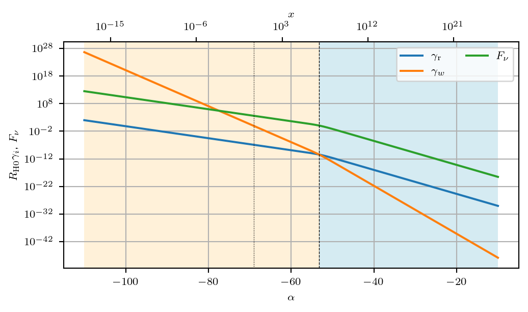
Adiabatic regime and truncation error
The adiabatic approximation relies on small correction factors for the mode functions and their conjugate momenta. A useful diagnostic is the product \(c_i F_\nu\): when \(c_i F_\nu\gg1\) a mode is deep inside the sub-Hubble (adiabatic) regime; when \(c_i F_\nu\ll1\) it is super-Hubble. The transition \(c_i F_\nu=1\) approximately marks the boundary of the adiabatic regime.
The simple \(c_i F_\nu\) test is only an estimate of the truncation error. In the code we compute a third-order truncation estimate (product of first- and second-order corrections) and compare its cubic root with \(c_i F_\nu\) to assess the quality of the adiabatic series.
Code
results = [Nc.HIPertITwoFluids.wkb_eval(cosmo_rw, alpha, k) for alpha in alpha_mode_a]

delta_zeta1 = np.array([res.mode1_zeta_scale for res in results])
delta_zeta2 = np.array([res.mode2_zeta_scale for res in results])
delta_Q1 = np.array([res.mode1_Q_scale for res in results])
delta_Q2 = np.array([res.mode2_Q_scale for res in results])
delta_Pzeta1 = np.array([res.mode1_Pzeta_scale for res in results])
delta_Pzeta2 = np.array([res.mode2_Pzeta_scale for res in results])
delta_PQ1 = np.array([res.mode1_PQ_scale for res in results])
delta_PQ2 = np.array([res.mode2_PQ_scale for res in results])

set_rc_params_article(ncol=1, nrows=1, aspect_ratio=0.5)
fig, ax = plt.subplots()

next_color = get_next_color()

scale_array = [
    (
        delta_zeta1,
        delta_zeta2,
        r"$\Delta_{\zeta_1} c_\mathrm{r} F_\nu$",
        r"$\Delta_{\zeta_2} c_w F_\nu$",
    ),
    (
        delta_Q1,
        delta_Q2,
        r"$\Delta_{Q_1} c_\mathrm{r} F_\nu$",
        r"$\Delta_{Q_2} c_w F_\nu$",
    ),
    (
        delta_Pzeta1,
        delta_Pzeta2,
        r"$\Delta_{\Pi{\zeta_1}} c_\mathrm{r} F_\nu$",
        r"$\Delta_{\Pi{\zeta_2}} c_w F_\nu$",
    ),
    (
        delta_PQ1,
        delta_PQ2,
        r"$\Delta_{\Pi{Q_1}} c_\mathrm{r} F_\nu$",
        r"$\Delta_{\Pi{Q_2}} c_w F_\nu$",
    ),
]

# Plot the truncation error
for delta1, delta2, label1, label2 in scale_array:
    c = next_color()
    ax.plot(
        alpha_mode_a, delta1 * c1 * Fnu, color=c, linestyle="-", lw=lw, label=label1
    )
    ax.plot(
        alpha_mode_a, delta2 * c2 * Fnu, color=c, linestyle="--", lw=lw, label=label2
    )

# Vertical markers
ax.axvline(x=alpha_eq, color="k", linestyle="dashed", lw=lw)
ax.axvline(x=alpha0, color="k", linestyle="dotted", lw=lw)

ax.axvspan(alpha_mode_ini, alpha_eq, **md)
ax.axvspan(alpha_eq, alpha_mode_end, **rd)

# Axis formatting
format_alpha_xaxis(ax, cosmo_rw)
# ax.set_yscale("log")
ax.set_ylabel(r"Adiabatic Scale Comparison")
ax.legend(ncol=2)
ax.grid()

# Save and show
plt.savefig(os.path.join(fig_dir, "truncation-error.pdf"), bbox_inches="tight")
fig.set_size_inches(6, 3)
plt.show()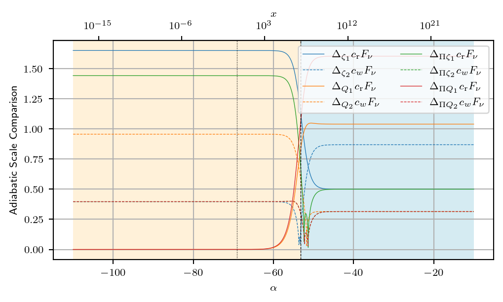
Note that the mode~2 variables (associated with the matter speed of sound \(c_w\)) usually have a smaller truncation error than the mode~1 passing closer to zero during the matter-radiation transition. It is useful to zoom in on the region around \(x_\mathrm{eq}\) to see the differences more clearly.
Code
alpha_zoom_ini = alpha_eq - 5.0
alpha_zoom_end = alpha_eq + 5.0

alpha_zoom_a = np.linspace(alpha_zoom_ini, alpha_zoom_end, 2000)
results_zoom = [
    Nc.HIPertITwoFluids.wkb_eval(cosmo_rw, alpha, k) for alpha in alpha_zoom_a
]
delta_zeta1 = np.array([res.mode1_zeta_scale for res in results_zoom])
delta_zeta2 = np.array([res.mode2_zeta_scale for res in results_zoom])
delta_Q1 = np.array([res.mode1_Q_scale for res in results_zoom])
delta_Q2 = np.array([res.mode2_Q_scale for res in results_zoom])
delta_Pzeta1 = np.array([res.mode1_Pzeta_scale for res in results_zoom])
delta_Pzeta2 = np.array([res.mode2_Pzeta_scale for res in results_zoom])
delta_PQ1 = np.array([res.mode1_PQ_scale for res in results_zoom])
delta_PQ2 = np.array([res.mode2_PQ_scale for res in results_zoom])
Fnu = np.array([res.state.Fnu for res in results_zoom])

set_rc_params_article(ncol=2, nrows=1, aspect_ratio=aspect2c)
fig, (ax1, ax2) = plt.subplots(ncols=2, nrows=1, sharex=True, sharey=True)

next_color = get_next_color()

scale_array = [
    (
        delta_zeta1,
        delta_zeta2,
        r"$\Delta_{\zeta_1} c_\mathrm{r} F_\nu$",
        r"$\Delta_{\zeta_2} c_w F_\nu$",
    ),
    (
        delta_Q1,
        delta_Q2,
        r"$\Delta_{Q_1} c_\mathrm{r} F_\nu$",
        r"$\Delta_{Q_2} c_w F_\nu$",
    ),
    (
        delta_Pzeta1,
        delta_Pzeta2 * 1.01,  # Slightly adjust to avoid overlap
        r"$\Delta_{\Pi{\zeta_1}} c_\mathrm{r} F_\nu$",
        r"$\Delta_{\Pi{\zeta_2}} c_w F_\nu$",
    ),
    (
        delta_PQ1,
        delta_PQ2,
        r"$\Delta_{\Pi{Q_1}} c_\mathrm{r} F_\nu$",
        r"$\Delta_{\Pi{Q_2}} c_w F_\nu$",
    ),
]
print(delta_Pzeta2)

# Plot the truncation error
for delta1, delta2, label1, label2 in scale_array:
    c = next_color()
    ax1.plot(
        alpha_zoom_a, delta1 * c1 * Fnu, color=c, linestyle="-", lw=lw, label=label1
    )
    ax2.plot(
        alpha_zoom_a, delta2 * c2 * Fnu, color=c, linestyle="--", lw=lw, label=label2
    )

# Vertical markers
ax1.axvline(x=alpha_eq, color="k", linestyle="dashed", lw=lw)
ax2.axvline(x=alpha_eq, color="k", linestyle="dashed", lw=lw)

ax1.axvspan(alpha_zoom_ini, alpha_eq, **md)
ax1.axvspan(alpha_eq, alpha_zoom_end, **rd)
ax2.axvspan(alpha_zoom_ini, alpha_eq, **md)
ax2.axvspan(alpha_eq, alpha_zoom_end, **rd)

# Axis formatting
format_alpha_xaxis(ax1, cosmo_rw)
format_alpha_xaxis(ax2, cosmo_rw)
ax1.set_ylabel(r"Adiabatic Scale Comparison")

ax1.legend(ncol=2, loc="upper left")
ax2.legend(ncol=2, loc="upper left")
ax1.grid()
ax2.grid()

# Save and show
plt.savefig(os.path.join(fig_dir, "truncation-error-zoom.pdf"), bbox_inches="tight")
fig.set_size_inches(12, 12 * aspect2c)
plt.show()
[2.09173765e+01 2.09701863e+01 2.10231314e+01 ... 2.50093193e+04
2.51378660e+04 2.52670572e+04]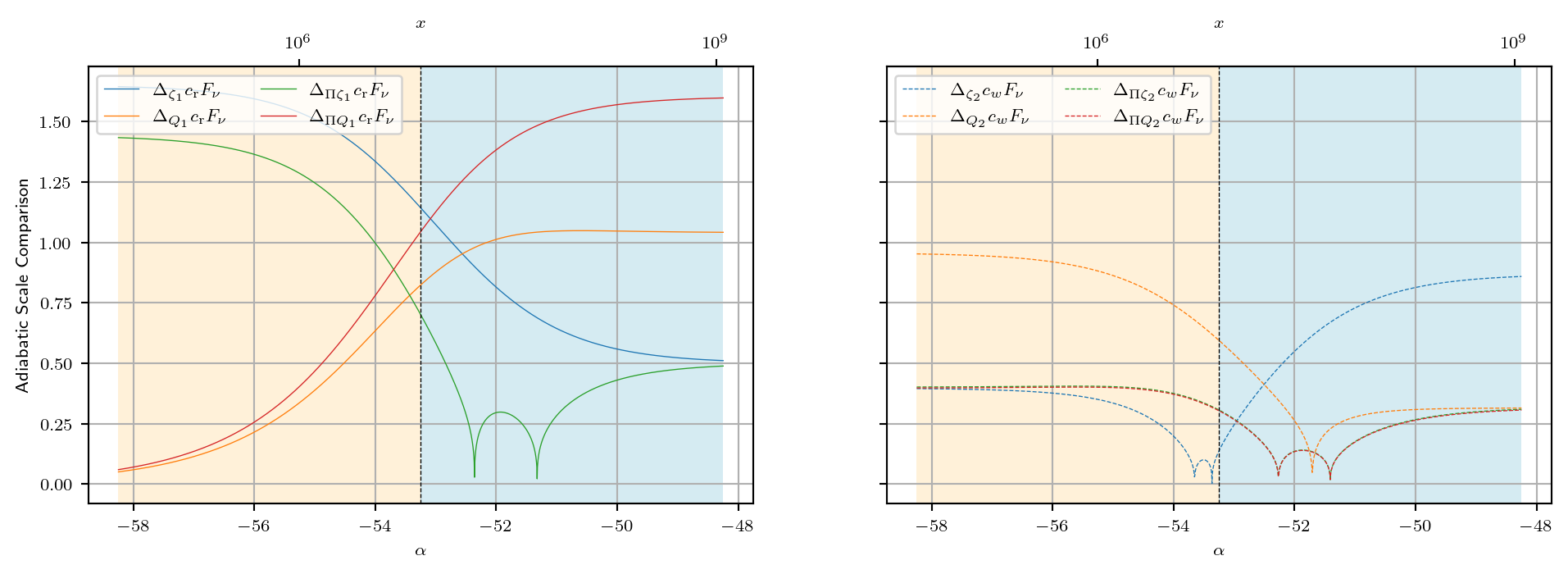
Evolving the Modes
To compute the power spectra, we use the HIPertTwoFluids object, which includes all perturbation components, such as matter and radiation. Initial conditions are set in the adiabatic vacuum state. The time where \(c_i F_\nu = 1\) also identifies the limit of validity for the adiabatic approximation for each mode.
pert = Nc.HIPertTwoFluids.new()
pert.props.reltol = reltol
pert.set_initial_time(alpha_ini_integ)
pert.set_final_time(alpha_end_integ)
pert.set_wkb_reltol(1.0e-3)

# Prepare a color map to depict the modes
norm = mpl.colors.LogNorm(vmin=1.0 / k_values.max(), vmax=1.0 / k_values.min())
sm = mpl.cm.ScalarMappable(norm=norm, cmap=cmap)

observables = [
    (Nc.HIPertITwoFluidsObs.ZETA, "zeta"),
    (Nc.HIPertITwoFluidsObs.ZETA_DIFF, "dzeta"),
    (Nc.HIPertITwoFluidsObs.DELTA_TOT, "delta_rho"),
    (Nc.HIPertITwoFluidsObs.DELTA_DIFF, "diff_delta_rho"),
    (Nc.HIPertITwoFluidsObs.PZETA, "pzeta"),
]

modes_list = []
modes_wkb_list = []
power_spectra_list = []

for k in k_values:
    lambda_com = 1.0 / k
    pert.set_mode_k(k * RH_Mpc)
    color = cmap(norm(lambda_com))
    modes = {}
    modes_wkb = {}
    power_spectra = {}

    s_interp = pert.evol_mode(cosmo_rw)

    for obs, name in observables:
        for mode, mode_str in [
            (Nc.HIPertITwoFluidsObsMode.ONE, "1"),
            (Nc.HIPertITwoFluidsObsMode.TWO, "2"),
        ]:
            modes[f"{name}{mode_str}"] = np.abs(
                [
                    s_interp.eval(cosmo_rw, alpha).eval_mode(mode, obs).Re()
                    for alpha in alpha_mode_a
                ]
            )
            modes_wkb[f"{name}{mode_str}"] = np.abs(
                [
                    Nc.HIPertITwoFluids.wkb_eval(cosmo_rw, alpha, k * RH_Mpc)
                    .peek_state()
                    .eval_mode(mode, obs)
                    .Abs()
                    for alpha in alpha_mode_a
                ]
            )

    for obs, obs_name in observables:
        for mode, mode_str in [
            (Nc.HIPertITwoFluidsObsMode.ONE, "1"),
            (Nc.HIPertITwoFluidsObsMode.TWO, "2"),
            (Nc.HIPertITwoFluidsObsMode.BOTH, ""),
        ]:
            power_spectra[f"{obs_name}{mode_str}"] = np.abs(
                [
                    s_interp.eval(cosmo_rw, alpha).eval_obs(mode, obs, obs)
                    for alpha in alpha_pk_a
                ]
            )

    modes_list.append(modes)
    modes_wkb_list.append(modes_wkb)
    power_spectra_list.append(power_spectra)


def find_single_crossing(x_a, y1_a, y2_a):
    """
    Finds the x-coordinate where y1_a and y2_a cross.
    Assumes they cross exactly once.
    """
    diff = y1_a - y2_a
    idx = np.where(np.sign(diff[:-1]) != np.sign(diff[1:]))[0][0]

    # Linear interpolation
    x0, x1 = x_a[idx], x_a[idx + 1]
    y0, y1 = diff[idx], diff[idx + 1]
    x_cross = x0 - y0 * (x1 - x0) / (y1 - y0)

    return x_cross
We can plot the mode evolution for mode \(k\in {k_\mathrm{min}, k_\mathrm{max}}\), each mode has two linearly independent solutions associated with creation and annihilation operators.
Code
set_rc_params_article(ncol=2, nrows=1, aspect_ratio=aspect2c2r)
fig, ((ax0, ax1), (ax2, ax3)) = plt.subplots(
    ncols=2, nrows=2, sharex=True, sharey="row"
)
fig.subplots_adjust(hspace=0.0, wspace=0.0)

c1_comoving_RH_a = c1 * (
    np.array(
        [
            Nc.HIPertITwoFluids.eom_eval(cosmo_rw, alpha, k).Fnu / k
            for alpha in alpha_mode_a
        ]
    )
    * RH_Mpc
)
c2_comoving_RH_a = c2 * (
    np.array(
        [
            Nc.HIPertITwoFluids.eom_eval(cosmo_rw, alpha, k).Fnu / k
            for alpha in alpha_mode_a
        ]
    )
    * RH_Mpc
)
first = True

for k, modes, modes_wkb in zip(k_values, modes_list, modes_wkb_list):
    lambda_com = 1.0 / k
    color = cmap(norm(lambda_com))

    alpha_cross1 = find_single_crossing(
        alpha_mode_a, c1_comoving_RH_a, np.ones_like(alpha_mode_a) * lambda_com
    )

    alpha_cross2 = find_single_crossing(
        alpha_mode_a, c2_comoving_RH_a, np.ones_like(alpha_mode_a) * lambda_com
    )

    ax2.plot(
        alpha_mode_a,
        modes["zeta1"] / k,
        linestyle="solid",
        lw=lw,
        color=color,
        label=r"$k^{-1}\zeta_1$" if first else None,
    )
    ax3.plot(
        alpha_mode_a,
        modes["zeta2"] / k,
        linestyle="solid",
        lw=lw,
        color=color,
        label=r"$k^{-1}\zeta_2$" if first else None,
    )
    ax2.plot(
        alpha_mode_a,
        modes_wkb["zeta1"] / k,
        linestyle="dashed",
        lw=lw,
        color=color,
        label=r"$k^{-1}\zeta_1^\mathrm{WKB}$" if first else None,
    )
    ax3.plot(
        alpha_mode_a,
        modes_wkb["zeta2"] / k,
        linestyle="dashed",
        lw=lw,
        color=color,
        label=r"$k^{-1}\zeta_2^\mathrm{WKB}$" if first else None,
    )

    ax0.axhline(
        lambda_com,
        linestyle="solid",
        lw=lw,
        color=color,
        label=r"$\lambda$" if first else None,
    )
    ax1.axhline(
        lambda_com,
        linestyle="solid",
        lw=lw,
        color=color,
        label=r"$\lambda$" if first else None,
    )

    ax0.axvline(x=alpha_cross1, linestyle="solid", lw=lw, color=color)
    ax2.axvline(x=alpha_cross1, linestyle="solid", lw=lw, color=color)

    ax1.axvline(x=alpha_cross2, linestyle="solid", lw=lw, color=color)
    ax3.axvline(x=alpha_cross2, linestyle="solid", lw=lw, color=color)
    first = False

ax0.plot(
    alpha_mode_a,
    c1_comoving_RH_a,
    linestyle="dashed",
    lw=lw,
    color="k",
    label=r"$c_\mathrm{r} x R_H$",
)
ax1.plot(
    alpha_mode_a,
    c2_comoving_RH_a,
    linestyle="dashed",
    lw=lw,
    color="k",
    label=r"$c_w x R_H$",
)

# Shaded dominance regions
for ax in (ax0, ax1, ax2, ax3):
    ax.axvspan(alpha_mode_ini, alpha_eq, **md)
    ax.axvspan(alpha_eq, alpha_mode_end, **rd)
    ax.set_yscale("log")
    ax.legend()

format_alpha_xaxis(ax0, cosmo_rw, bottom=False)
format_alpha_xaxis(ax2, cosmo_rw, top=False)
format_alpha_xaxis(ax1, cosmo_rw, bottom=False)
format_alpha_xaxis(ax3, cosmo_rw, top=False)

ax0.set_ylabel(r"$\lambda$, $c_s x R_H$ [Mpc]")
ax2.set_ylabel(r"$k^{-1}\zeta_i$")

# Colorbar for k
cbar = fig.colorbar(sm, ax=[ax0, ax1, ax2, ax3], pad=0.02)
cbar.set_label(r"$\lambda$ [Mpc]")

# Save and show
plt.savefig(os.path.join(fig_dir, "mode_zeta_evolution.pdf"), bbox_inches="tight")
fig.set_size_inches(12, 12 * aspect2c2r)

plt.show()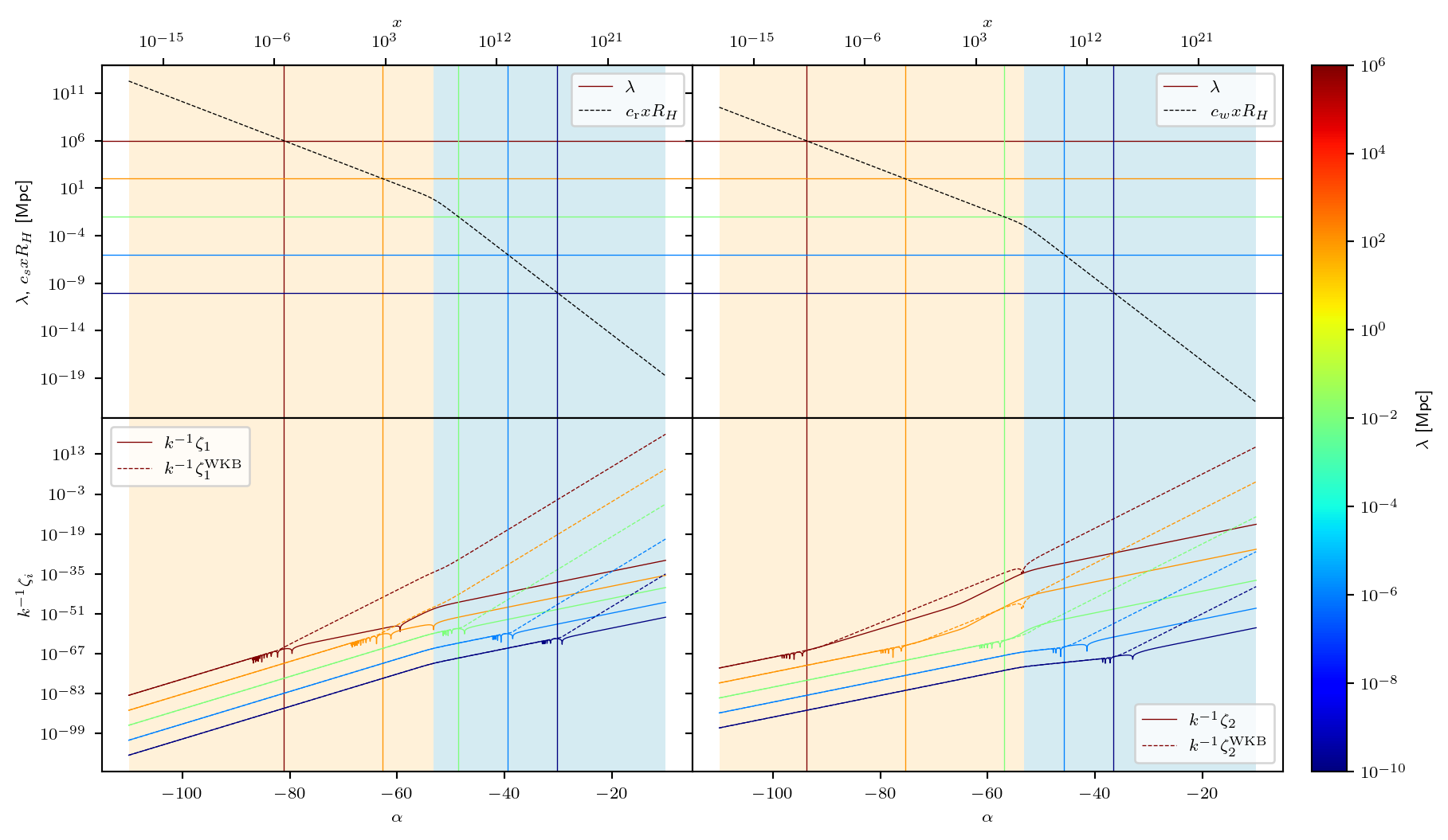
Now we can do the same for the entropy perturbation \(Q_i \propto \Delta\zeta_i \equiv \zeta_{\mathrm{r}i} - \zeta_{w i}\), which is the difference between the radiation and matter modes.
Code
set_rc_params_article(ncol=2, nrows=1, aspect_ratio=aspect2c2r)
fig, ((ax0, ax1), (ax2, ax3)) = plt.subplots(
    ncols=2, nrows=2, sharex=True, sharey="row"
)
fig.subplots_adjust(hspace=0.0, wspace=0.0)

first = True

for k, modes, modes_wkb in zip(k_values, modes_list, modes_wkb_list):
    lambda_com = 1.0 / k
    color = cmap(norm(lambda_com))

    alpha_cross1 = find_single_crossing(
        alpha_mode_a, c1_comoving_RH_a, np.ones_like(alpha_mode_a) * lambda_com
    )
    alpha_cross2 = find_single_crossing(
        alpha_mode_a, c2_comoving_RH_a, np.ones_like(alpha_mode_a) * lambda_com
    )

    ax2.plot(
        alpha_mode_a,
        modes["dzeta1"] / k,
        linestyle="solid",
        lw=lw,
        color=color,
        label=r"$k^{-1}\Delta\zeta_1$" if first else None,
    )
    ax3.plot(
        alpha_mode_a,
        modes["dzeta2"] / k,
        linestyle="solid",
        lw=lw,
        color=color,
        label=r"$k^{-1}\Delta\zeta_2$" if first else None,
    )

    # Now the WKB approximation

    ax2.plot(
        alpha_mode_a,
        modes_wkb["dzeta1"] / k,
        linestyle="dashed",
        lw=lw,
        color=color,
        label=r"$k^{-1}\Delta\zeta_1^\mathrm{WKB}$" if first else None,
    )
    ax3.plot(
        alpha_mode_a,
        modes_wkb["dzeta2"] / k,
        linestyle="dashed",
        lw=lw,
        color=color,
        label=r"$k^{-1}\Delta\zeta_2^\mathrm{WKB}$" if first else None,
    )

    ax0.axhline(
        lambda_com,
        linestyle="solid",
        lw=lw,
        color=color,
        label=r"$\lambda$" if first else None,
    )
    ax1.axhline(
        lambda_com,
        linestyle="solid",
        lw=lw,
        color=color,
        label=r"$\lambda$" if first else None,
    )

    ax0.axvline(x=alpha_cross1, linestyle="solid", lw=lw, color=color)
    ax2.axvline(x=alpha_cross1, linestyle="solid", lw=lw, color=color)
    ax1.axvline(x=alpha_cross2, linestyle="solid", lw=lw, color=color)
    ax3.axvline(x=alpha_cross2, linestyle="solid", lw=lw, color=color)

    first = False

ax0.plot(
    alpha_mode_a,
    c1_comoving_RH_a,
    linestyle="dashed",
    lw=lw,
    color="k",
    label=r"$c_\mathrm{r} x R_H$",
)
ax1.plot(
    alpha_mode_a,
    c2_comoving_RH_a,
    linestyle="dashed",
    lw=lw,
    color="k",
    label=r"$c_w x R_H$",
)

for ax in (ax0, ax1, ax2, ax3):
    ax.axvspan(alpha_mode_ini, alpha_eq, **md)
    ax.axvspan(alpha_eq, alpha_mode_end, **rd)
    ax.set_yscale("log")
    ax.legend()

format_alpha_xaxis(ax0, cosmo_rw, bottom=False)
format_alpha_xaxis(ax2, cosmo_rw, top=False)
format_alpha_xaxis(ax1, cosmo_rw, bottom=False)
format_alpha_xaxis(ax3, cosmo_rw, top=False)

ax0.set_ylabel(r"$\lambda$, $c_s x R_H$ [Mpc]")
ax2.set_ylabel(r"$k^{-1}\Delta\zeta_i$")

# Colorbar for k
cbar = fig.colorbar(sm, ax=[ax0, ax1, ax2, ax3], pad=0.02)
cbar.set_label(r"$\lambda$ [Mpc]")

# Save and show
plt.savefig(os.path.join(fig_dir, "mode_dzeta_evolution.pdf"), bbox_inches="tight")
fig.set_size_inches(12, 12 * aspect2c2r)

plt.show()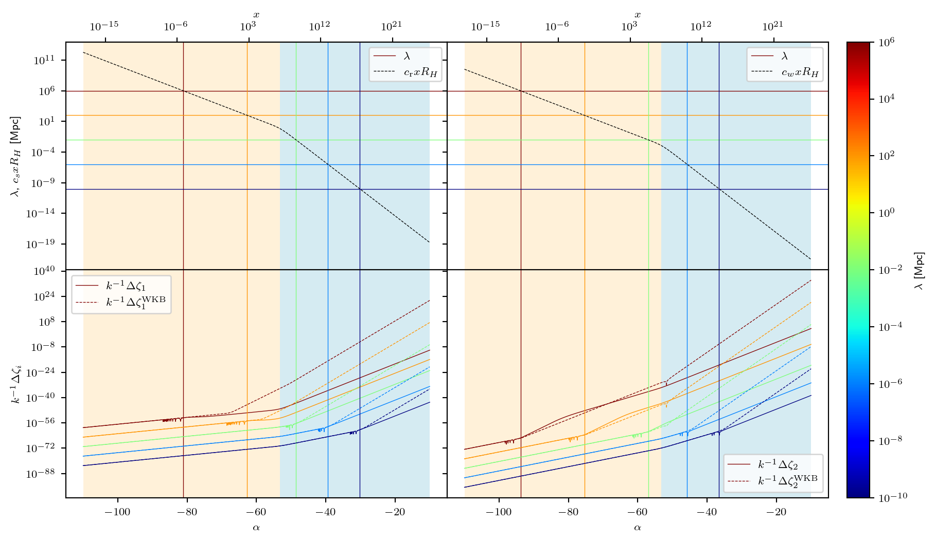
Next we can plot the density perturbations \(\bar{\delta}_{\rho i}\) for each mode.
Code
set_rc_params_article(ncol=2, nrows=1, aspect_ratio=aspect2c2r)
fig, ((ax0, ax1), (ax2, ax3)) = plt.subplots(
    ncols=2, nrows=2, sharex=True, sharey="row"
)
fig.subplots_adjust(hspace=0.0, wspace=0.0)

first = True

for k, modes, modes_wkb in zip(k_values, modes_list, modes_wkb_list):
    lambda_com = 1.0 / k
    color = cmap(norm(lambda_com))

    alpha_cross1 = find_single_crossing(
        alpha_mode_a, c1_comoving_RH_a, np.ones_like(alpha_mode_a) * lambda_com
    )
    alpha_cross2 = find_single_crossing(
        alpha_mode_a, c2_comoving_RH_a, np.ones_like(alpha_mode_a) * lambda_com
    )

    ax2.plot(
        alpha_mode_a,
        modes["delta_rho1"] / k,
        linestyle="solid",
        lw=lw,
        color=color,
        label=r"$k^{-1}\bar{\delta}_{\rho 1}$" if first else None,
    )
    ax3.plot(
        alpha_mode_a,
        modes["delta_rho2"] / k,
        linestyle="solid",
        lw=lw,
        color=color,
        label=r"$k^{-1}\bar{\delta}_{\rho 2}$" if first else None,
    )

    ax2.plot(
        alpha_mode_a,
        modes_wkb["delta_rho1"] / k,
        linestyle="dashed",
        lw=lw,
        color=color,
        label=r"$k^{-1}\bar{\delta}_{\rho 1}^\mathrm{WKB}$" if first else None,
    )
    ax3.plot(
        alpha_mode_a,
        modes_wkb["delta_rho2"] / k,
        linestyle="dashed",
        lw=lw,
        color=color,
        label=r"$k^{-1}\bar{\delta}_{\rho 2}^\mathrm{WKB}$" if first else None,
    )

    ax0.axhline(
        lambda_com,
        linestyle="solid",
        lw=lw,
        color=color,
        label=r"$\lambda$" if first else None,
    )
    ax1.axhline(
        lambda_com,
        linestyle="solid",
        lw=lw,
        color=color,
        label=r"$\lambda$" if first else None,
    )

    ax0.axvline(x=alpha_cross1, linestyle="solid", lw=lw, color=color)
    ax2.axvline(x=alpha_cross1, linestyle="solid", lw=lw, color=color)
    ax1.axvline(x=alpha_cross2, linestyle="solid", lw=lw, color=color)
    ax3.axvline(x=alpha_cross2, linestyle="solid", lw=lw, color=color)

    first = False

ax0.plot(
    alpha_mode_a,
    c1_comoving_RH_a,
    linestyle="dashed",
    lw=lw,
    color="k",
    label=r"$c_\mathrm{r} x R_H$",
)
ax1.plot(
    alpha_mode_a,
    c2_comoving_RH_a,
    linestyle="dashed",
    lw=lw,
    color="k",
    label=r"$c_w x R_H$",
)

for ax in (ax0, ax1, ax2, ax3):
    ax.axvspan(alpha_mode_ini, alpha_eq, **md)
    ax.axvspan(alpha_eq, alpha_mode_end, **rd)
    ax.set_yscale("log")
    ax.legend()

format_alpha_xaxis(ax0, cosmo_rw, bottom=False)
format_alpha_xaxis(ax2, cosmo_rw, top=False)
format_alpha_xaxis(ax1, cosmo_rw, bottom=False)
format_alpha_xaxis(ax3, cosmo_rw, top=False)

ax0.set_ylabel(r"$\lambda$, $c_s x R_H$ [Mpc]")
ax2.set_ylabel(r"$k^{-1}\bar{\delta}_{\rho i}$")
# Colorbar for k
cbar = fig.colorbar(sm, ax=[ax0, ax1, ax2, ax3], pad=0.02)
cbar.set_label(r"$\lambda$ [Mpc]")

# Save and show
plt.savefig(os.path.join(fig_dir, "mode_drho_evolution.pdf"), bbox_inches="tight")
fig.set_size_inches(12, 12 * aspect2c2r)

plt.show()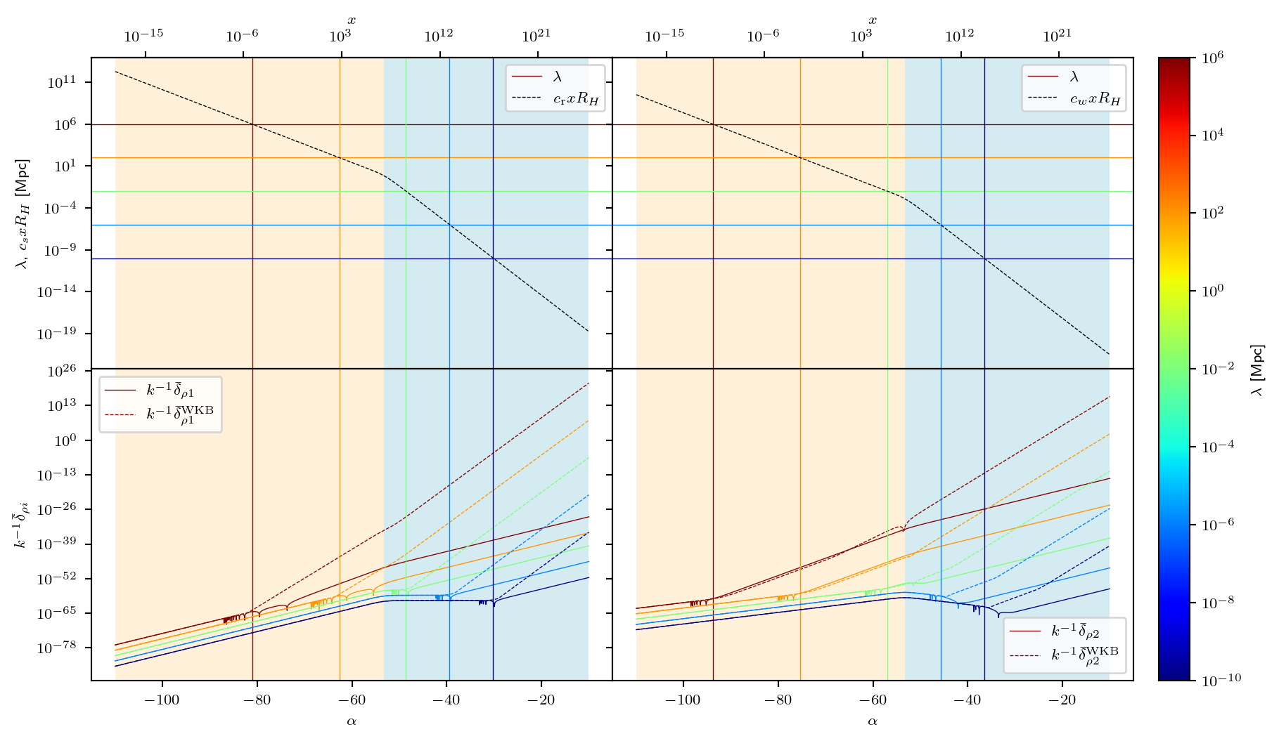
Finally, we can plot the difference in density perturbations \(\Delta\delta_{\rho i} = \delta_{\rho_{\mathrm{r}}i} - \delta_{\rho_{w}i}\) for each mode.
Code
set_rc_params_article(ncol=2, nrows=1, aspect_ratio=aspect2c2r)
fig, ((ax0, ax1), (ax2, ax3)) = plt.subplots(
    ncols=2, nrows=2, sharex=True, sharey="row"
)
fig.subplots_adjust(hspace=0.0, wspace=0.0)

first = True

for k, modes, modes_wkb in zip(k_values, modes_list, modes_wkb_list):
    lambda_com = 1.0 / k
    color = cmap(norm(lambda_com))

    alpha_cross1 = find_single_crossing(
        alpha_mode_a, c1_comoving_RH_a, np.ones_like(alpha_mode_a) * lambda_com
    )
    alpha_cross2 = find_single_crossing(
        alpha_mode_a, c2_comoving_RH_a, np.ones_like(alpha_mode_a) * lambda_com
    )

    ax2.plot(
        alpha_mode_a,
        modes["diff_delta_rho1"] / k,
        linestyle="solid",
        lw=lw,
        color=color,
        label=r"$k^{-1}\Delta\delta_{\rho 1}$" if first else None,
    )
    ax3.plot(
        alpha_mode_a,
        modes["diff_delta_rho2"] / k,
        linestyle="solid",
        lw=lw,
        color=color,
        label=r"$k^{-1}\Delta\delta_{\rho 2}$" if first else None,
    )

    ax2.plot(
        alpha_mode_a,
        modes_wkb["diff_delta_rho1"] / k,
        linestyle="dashed",
        lw=lw,
        color=color,
        label=r"$k^{-1}\Delta\delta_{\rho 1}^\mathrm{WKB}$" if first else None,
    )
    ax3.plot(
        alpha_mode_a,
        modes_wkb["diff_delta_rho2"] / k,
        linestyle="dashed",
        lw=lw,
        color=color,
        label=r"$k^{-1}\Delta\delta_{\rho 2}^\mathrm{WKB}$" if first else None,
    )

    ax0.axhline(
        lambda_com,
        linestyle="solid",
        lw=lw,
        color=color,
        label=r"$\lambda$" if first else None,
    )
    ax1.axhline(
        lambda_com,
        linestyle="solid",
        lw=lw,
        color=color,
        label=r"$\lambda$" if first else None,
    )

    ax0.axvline(x=alpha_cross1, linestyle="solid", lw=lw, color=color)
    ax2.axvline(x=alpha_cross1, linestyle="solid", lw=lw, color=color)
    ax1.axvline(x=alpha_cross2, linestyle="solid", lw=lw, color=color)
    ax3.axvline(x=alpha_cross2, linestyle="solid", lw=lw, color=color)

    first = False

ax0.plot(
    alpha_mode_a,
    c1_comoving_RH_a,
    linestyle="dashed",
    lw=lw,
    color="k",
    label=r"$c_\mathrm{r} x R_H$",
)
ax1.plot(
    alpha_mode_a,
    c2_comoving_RH_a,
    linestyle="dashed",
    lw=lw,
    color="k",
    label=r"$c_w x R_H$",
)

for ax in (ax0, ax1, ax2, ax3):
    ax.axvspan(alpha_mode_ini, alpha_eq, **md)
    ax.axvspan(alpha_eq, alpha_mode_end, **rd)
    ax.set_yscale("log")
    ax.legend()

format_alpha_xaxis(ax0, cosmo_rw, bottom=False)
format_alpha_xaxis(ax2, cosmo_rw, top=False)
format_alpha_xaxis(ax1, cosmo_rw, bottom=False)
format_alpha_xaxis(ax3, cosmo_rw, top=False)

ax0.set_ylabel(r"$\lambda$, $c_s x R_H$ [Mpc]")
ax2.set_ylabel(r"$k^{-1}\Delta\delta_{\rho i}$")
# Colorbar for k
cbar = fig.colorbar(sm, ax=[ax0, ax1, ax2, ax3], pad=0.02)
cbar.set_label(r"$\lambda$ [Mpc]")
# Save and show
plt.savefig(
    os.path.join(fig_dir, "mode_diff_delta_rho_evolution.pdf"), bbox_inches="tight"
)
fig.set_size_inches(12, 12 * aspect2c2r)
plt.show()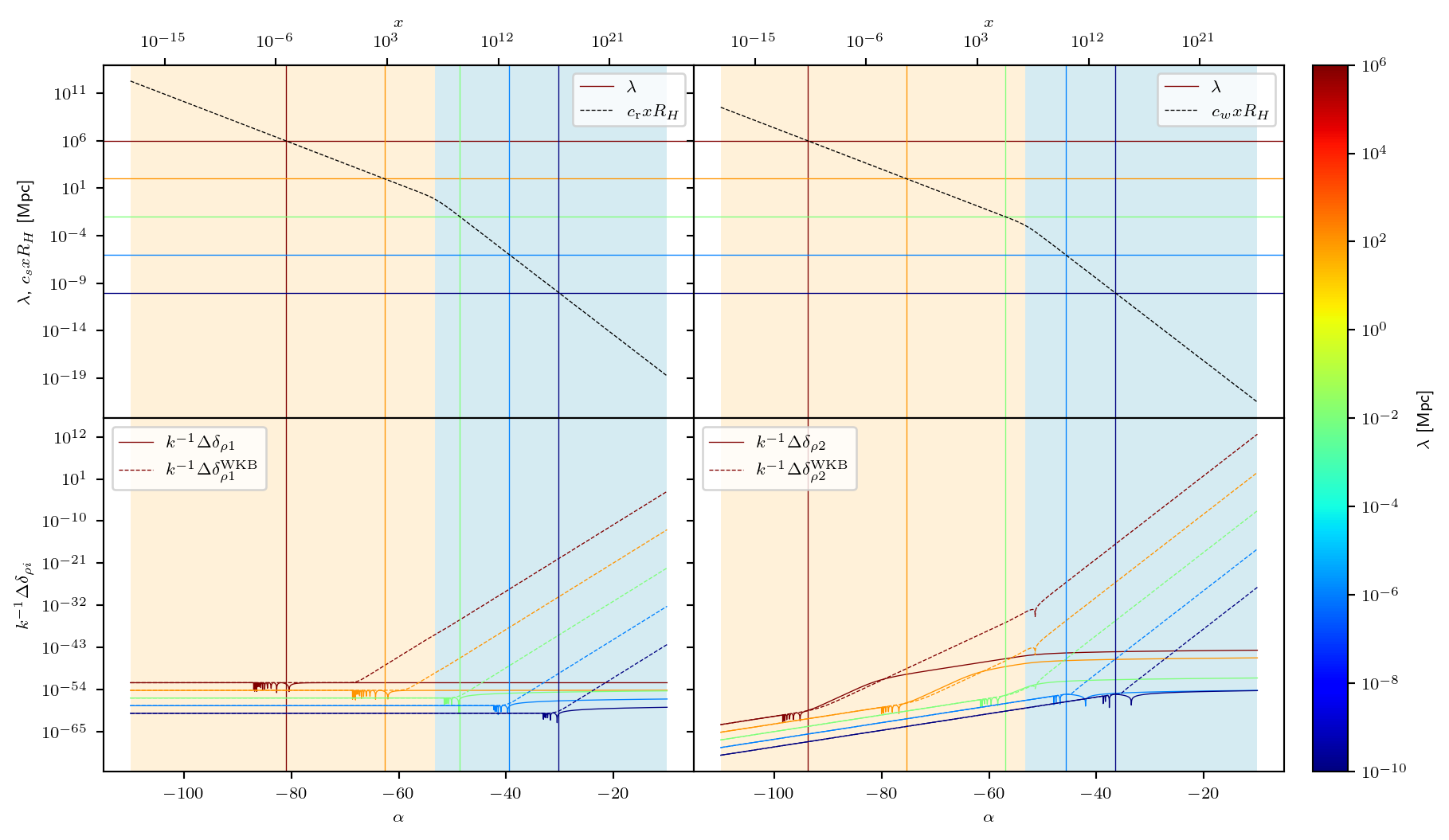
For completeness, we also plot the evolution of the momentum of the curvature perturbation:
Code
set_rc_params_article(ncol=2, nrows=1, aspect_ratio=aspect2c2r)
fig, ((ax0, ax1), (ax2, ax3)) = plt.subplots(
    ncols=2, nrows=2, sharex=True, sharey="row"
)
fig.subplots_adjust(hspace=0.0, wspace=0.0)

first = True

for k, modes, modes_wkb in zip(k_values, modes_list, modes_wkb_list):
    lambda_com = 1.0 / k
    color = cmap(norm(lambda_com))

    alpha_cross1 = find_single_crossing(
        alpha_mode_a, c1_comoving_RH_a, np.ones_like(alpha_mode_a) * lambda_com
    )
    alpha_cross2 = find_single_crossing(
        alpha_mode_a, c2_comoving_RH_a, np.ones_like(alpha_mode_a) * lambda_com
    )

    ax2.plot(
        alpha_mode_a,
        modes["pzeta1"] / k,
        linestyle="solid",
        lw=lw,
        color=color,
        label=r"$k^{-1}\Pi_{\zeta 1}$" if first else None,
    )
    ax3.plot(
        alpha_mode_a,
        modes["pzeta2"] / k,
        linestyle="solid",
        lw=lw,
        color=color,
        label=r"$k^{-1}\Pi_{\zeta 2}$" if first else None,
    )

    ax2.plot(
        alpha_mode_a,
        modes_wkb["pzeta1"] / k,
        linestyle="dashed",
        lw=lw,
        color=color,
        label=r"$k^{-1}\Pi_{\zeta 1}^\mathrm{WKB}$" if first else None,
    )
    ax3.plot(
        alpha_mode_a,
        modes_wkb["pzeta2"] / k,
        linestyle="dashed",
        lw=lw,
        color=color,
        label=r"$k^{-1}\Pi_{\zeta 2}^\mathrm{WKB}$" if first else None,
    )

    ax0.axhline(
        lambda_com,
        linestyle="solid",
        lw=lw,
        color=color,
        label=r"$\lambda$" if first else None,
    )
    ax1.axhline(
        lambda_com,
        linestyle="solid",
        lw=lw,
        color=color,
        label=r"$\lambda$" if first else None,
    )

    ax0.axvline(x=alpha_cross1, linestyle="solid", lw=lw, color=color)
    ax2.axvline(x=alpha_cross1, linestyle="solid", lw=lw, color=color)
    ax1.axvline(x=alpha_cross2, linestyle="solid", lw=lw, color=color)
    ax3.axvline(x=alpha_cross2, linestyle="solid", lw=lw, color=color)

    first = False

ax0.set_ylabel(r"$\lambda$ [Mpc]")
ax2.set_ylabel(r"$k^{-1}\Pi_{\zeta 1}$")

for ax in (ax0, ax1, ax2, ax3):
    ax.axvspan(alpha_mode_ini, alpha_eq, **md)
    ax.axvspan(alpha_eq, alpha_mode_end, **rd)
    ax.set_yscale("log")
    ax.legend()

format_alpha_xaxis(ax0, cosmo_rw, bottom=False)
format_alpha_xaxis(ax2, cosmo_rw, top=False)
format_alpha_xaxis(ax1, cosmo_rw, bottom=False)
format_alpha_xaxis(ax3, cosmo_rw, top=False)

ax0.set_xlabel(r"$\alpha$ [Mpc]")
ax2.set_xlabel(r"$\alpha$ [Mpc]")
ax1.set_xlabel(r"$\alpha$ [Mpc]")
ax3.set_xlabel(r"$\alpha$ [Mpc]")

# Colorbar for k
cbar = fig.colorbar(sm, ax=[ax0, ax1, ax2, ax3], pad=0.02)
cbar.set_label(r"$\lambda$ [Mpc]")
# Save and show
plt.savefig(os.path.join(fig_dir, "mode_pzeta_evolution.pdf"), bbox_inches="tight")
fig.set_size_inches(12, 12 * aspect2c2r)
plt.show()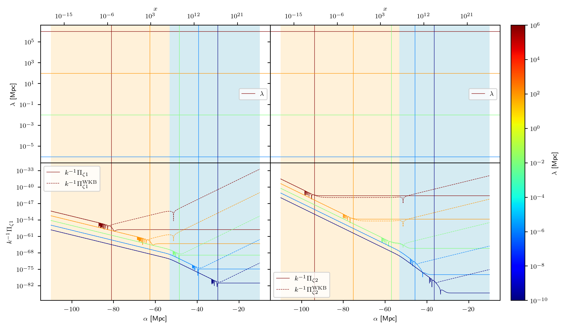
Power Spectra
The power spectra are computed using the HIPertTwoFluids object, which includes all perturbation components, such as matter and radiation. The initial conditions are set in the adiabatic vacuum state. We can now plot the evolution of the dimensionless power spectra for each mode. We already have computed all power spectra for the observables of interest, which are stored in the power_spectra_list variable. We denote the dimensionless power spectrum for mode \(X\) by \[
\mathcal{P}_X \equiv k^3 P_X, \qquad P_X \equiv \frac{\left\vert X \right\vert^2}{2\pi^2}.
\]
Now we plot the power spectrum time evolution for \(\zeta_i\). The figure shows the two mode spectra (\(\zeta_1\) left, \(\zeta_2\) right). A dotted horizontal line marks the large-scale approximation; shaded regions indicate radiation- and matter-dominated eras.
Code
set_rc_params_article(ncol=2, nrows=1, aspect_ratio=aspect2c)

fig, (ax0, ax1) = plt.subplots(ncols=2, nrows=1, sharey=True)
fig.subplots_adjust(hspace=0.0, wspace=0.0)

for k, power_spectra in zip(k_values, power_spectra_list):
    lambda_com = 1.0 / k
    color = cmap(norm(lambda_com))

    ax0.plot(
        alpha_pk_a,
        k**3 * RH_Mpc**3 * power_spectra["zeta1"],
        lw=lw,
        linestyle="solid",
        color=color,
        label=r"$\mathcal{P}_{\zeta_1}$" if k == k_values[0] else None,
    )
    ax1.plot(
        alpha_pk_a,
        k**3 * RH_Mpc**3 * power_spectra["zeta2"],
        lw=lw,
        linestyle="dashed",
        color=color,
        label=r"$\mathcal{P}_{\zeta_2}$" if k == k_values[0] else None,
    )

ax0.set_ylabel(r"$\mathcal{P}_{\zeta_i}$")

# Shaded dominance regions
for ax in (ax0, ax1):
    ax.axvspan(alpha_pk_ini, alpha_eq, **md)
    ax.axvspan(alpha_eq, alpha_pk_end, **rd)
    ax.axhline(large_scale_P_zeta(RH_Mpc), lw=lw, color="k", linestyle="dotted")
    ax.set_yscale("log")
    ax.legend()
    format_alpha_xaxis(ax, cosmo_rw)
    ax.set_xlabel(r"$\alpha$")
    ax.grid()

# Colorbar for k
cbar = fig.colorbar(sm, ax=(ax0, ax1), pad=0.02)
cbar.set_label(r"$\lambda$ [Mpc]")

fig.savefig(os.path.join(fig_dir, "zeta_power_spectrum.pdf"), bbox_inches="tight")

fig.set_size_inches(12, 12 * aspect2c)
plt.show()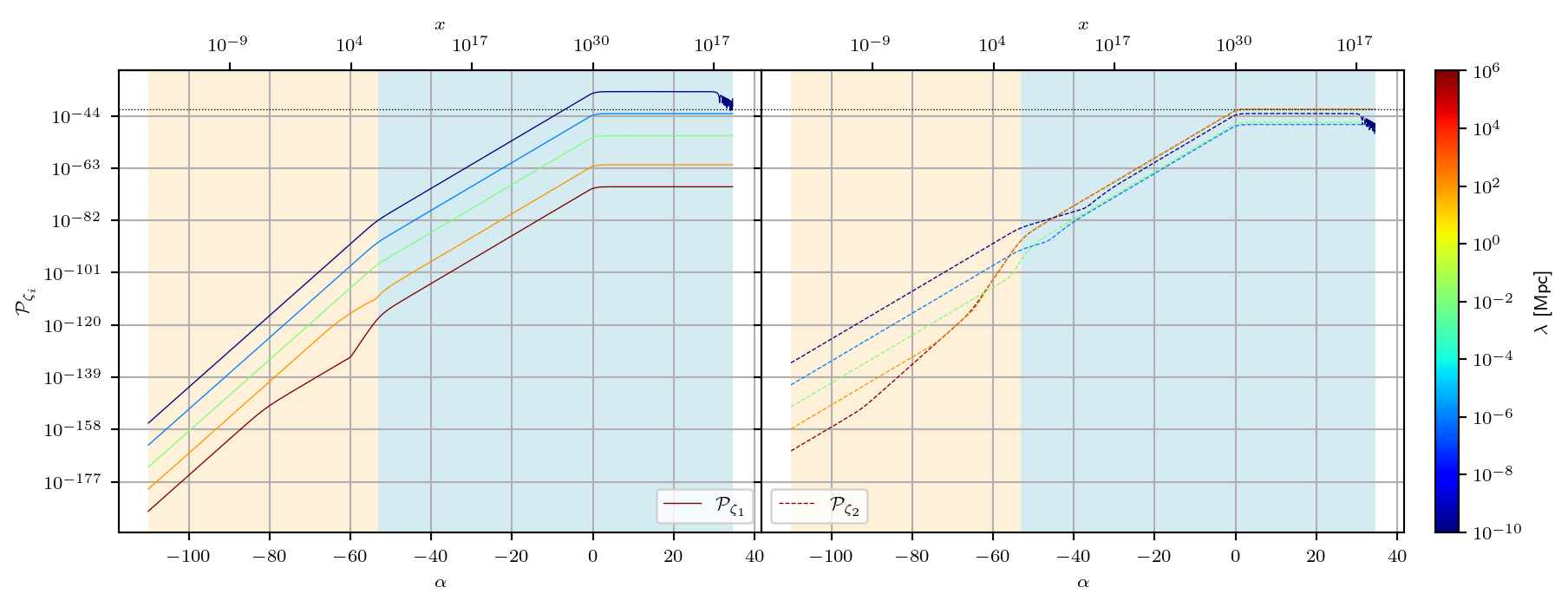
Now we plot the power spectrum time evolution for \(\Pi_{\zeta i}\):
Code
set_rc_params_article(ncol=2, nrows=1, aspect_ratio=aspect2c)

fig, (ax0, ax1) = plt.subplots(ncols=2, nrows=1, sharey=True)
fig.subplots_adjust(hspace=0.0, wspace=0.0)

for k, power_spectra in zip(k_values, power_spectra_list):
    lambda_com = 1.0 / k
    color = cmap(norm(lambda_com))

    ax0.plot(
        alpha_pk_a,
        k**3 * RH_Mpc**3 * power_spectra["pzeta1"],
        lw=lw,
        linestyle="solid",
        color=color,
        label=r"$\mathcal{P}_{\Pi_{\zeta 1}}$" if k == k_values[0] else None,
    )
    ax1.plot(
        alpha_pk_a,
        k**3 * RH_Mpc**3 * power_spectra["pzeta2"],
        lw=lw,
        linestyle="dashed",
        color=color,
        label=r"$\mathcal{P}_{\Pi_{\zeta 2}}$" if k == k_values[0] else None,
    )

ax0.set_ylabel(r"$\mathcal{P}_{\Pi_{\zeta i}}$")

# Shaded dominance regions
for ax in (ax0, ax1):
    ax.axvspan(alpha_pk_ini, alpha_eq, **md)
    ax.axvspan(alpha_eq, alpha_pk_end, **rd)
    ax.axhline(large_scale_P_zeta(RH_Mpc), lw=lw, color="k", linestyle="dotted")
    ax.set_yscale("log")
    ax.legend()
    format_alpha_xaxis(ax, cosmo_rw)
    ax.set_xlabel(r"$\alpha$")
    ax.grid()

# Colorbar for k
cbar = fig.colorbar(sm, ax=(ax0, ax1), pad=0.02)
cbar.set_label(r"$\lambda$ [Mpc]")

fig.savefig(os.path.join(fig_dir, "pzeta_power_spectrum.pdf"), bbox_inches="tight")

fig.set_size_inches(12, 12 * aspect2c)
plt.show()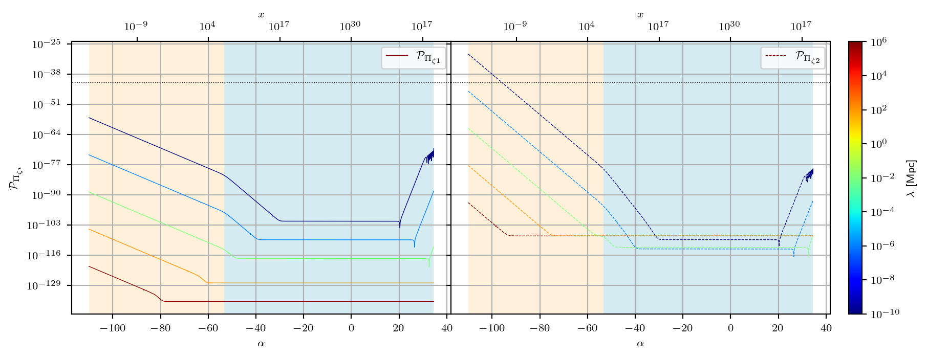
Now we can plot the power spectrum time evolution for \(\Delta\zeta_i\):
Code
set_rc_params_article(ncol=2, nrows=1, aspect_ratio=aspect2c)

fig, (ax0, ax1) = plt.subplots(ncols=2, nrows=1, sharey=True)
fig.subplots_adjust(hspace=0.0, wspace=0.0)

for k, power_spectra in zip(k_values, power_spectra_list):
    lambda_com = 1.0 / k
    color = cmap(norm(lambda_com))

    ax0.plot(
        alpha_pk_a,
        k**3 * RH_Mpc**3 * power_spectra["dzeta1"],
        lw=lw,
        linestyle="solid",
        color=color,
        label=r"$\mathcal{P}_{\Delta\zeta_1}$" if k == k_values[0] else None,
    )
    ax1.plot(
        alpha_pk_a,
        k**3 * RH_Mpc**3 * power_spectra["dzeta2"],
        lw=lw,
        linestyle="dashed",
        color=color,
        label=r"$\mathcal{P}_{\Delta\zeta_2}$" if k == k_values[0] else None,
    )

ax0.set_ylabel(r"$\mathcal{P}_{\Delta\zeta_i}$")

# Shaded dominance regions
for ax in (ax0, ax1):
    ax.axvspan(alpha_pk_ini, alpha_eq, **md)
    ax.axvspan(alpha_eq, alpha_pk_end, **rd)
    ax.set_yscale("log")
    ax.legend()
    format_alpha_xaxis(ax, cosmo_rw)
    ax.set_xlabel(r"$\alpha$")
    ax.grid()

# Colorbar for k
cbar = fig.colorbar(sm, ax=(ax0, ax1), pad=0.02)
cbar.set_label(r"$\lambda$ [Mpc]")

fig.savefig(os.path.join(fig_dir, "delta_zeta_power_spectrum.pdf"), bbox_inches="tight")

fig.set_size_inches(12, 12 * aspect2c)
plt.show()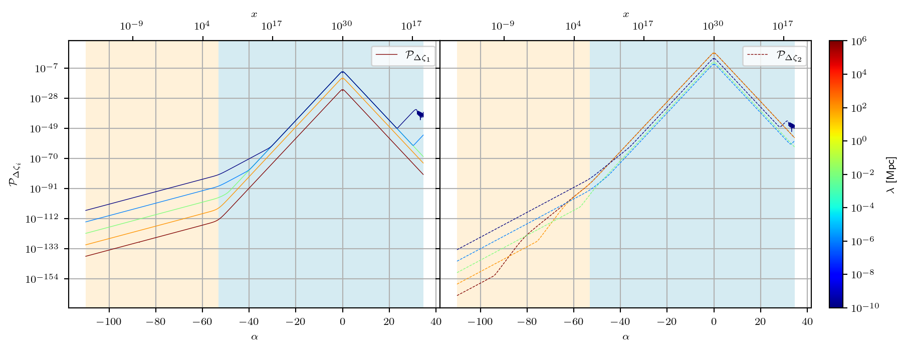
Now that we have seen the evolution of each adiabatic perturbation \(\zeta_i\) and \(\Delta\zeta_i\), we can plot the evolution of the total \(\zeta\) as well as the entropy perturbation \(\Delta\zeta = (\zeta_{\mathrm{r}} - \zeta_{w})\).
Code
set_rc_params_article(ncol=2, nrows=1, aspect_ratio=aspect2c)

fig, (ax0, ax1) = plt.subplots(ncols=2, nrows=1, sharey=True)
fig.subplots_adjust(hspace=0.0, wspace=0.0)

for k, power_spectra in zip(k_values, power_spectra_list):
    lambda_com = 1.0 / k
    color = cmap(norm(lambda_com))

    ax0.plot(
        alpha_pk_a,
        k**3 * RH_Mpc**3 * power_spectra["zeta"],
        lw=lw,
        linestyle="solid",
        color=color,
        label=r"$\mathcal{P}_{\zeta}$" if k == k_values[0] else None,
    )
ax0.set_ylabel(r"$\mathcal{P}_{\zeta}$, $\mathcal{P}_{\Delta\zeta}$")

# Shaded dominance regions
ax0.axvspan(alpha_pk_ini, alpha_eq, **md)
ax0.axvspan(alpha_eq, alpha_pk_end, **rd)
ax0.set_yscale("log")
ax0.legend()
format_alpha_xaxis(ax0, cosmo_rw)
ax0.set_xlabel(r"$\alpha$")
ax0.grid()

for k, power_spectra in zip(k_values, power_spectra_list):
    lambda_com = 1.0 / k
    color = cmap(norm(lambda_com))

    ax1.plot(
        alpha_pk_a,
        k**3 * RH_Mpc**3 * power_spectra["dzeta"],
        lw=lw,
        linestyle="solid",
        color=color,
        label=r"$\mathcal{P}_{\Delta\zeta}$" if k == k_values[0] else None,
    )

# Shaded dominance regions
ax1.axvspan(alpha_pk_ini, alpha_eq, **md)
ax1.axvspan(alpha_eq, alpha_pk_end, **rd)
ax1.set_yscale("log")
ax1.legend()
format_alpha_xaxis(ax1, cosmo_rw)
ax1.set_xlabel(r"$\alpha$")
ax1.grid()

# Report the maximum values at the bounce for both spectra
max_report = []
for k, power_spectra in zip(k_values, power_spectra_list):
    P_zeta = k**3 * RH_Mpc**3 * power_spectra["zeta"]
    P_dzeta = k**3 * RH_Mpc**3 * power_spectra["dzeta"]
    idx_zeta = np.argmax(P_zeta)
    idx_dzeta = np.argmax(P_dzeta)
    max_report.append(
        f"k = {k:.3e} Mpc^-1: "
        f"max P_zeta = {P_zeta[idx_zeta]:.3e} at alpha = {alpha_pk_a[idx_zeta]:.3f}; "
        f"max P_dzeta = {P_dzeta[idx_dzeta]:.3e} at alpha = {alpha_pk_a[idx_dzeta]:.3f}"
    )
print("Maximum power at the bounce for each mode:")
for line in max_report:
    print(line)

# Colorbar for k
cbar = fig.colorbar(sm, ax=ax1, pad=0.02)
cbar.set_label(r"$\lambda$ [Mpc]")

fig.savefig(os.path.join(fig_dir, "zeta_total_power_spectrum.pdf"), bbox_inches="tight")

fig.set_size_inches(12, 12 * aspect2c)
plt.show()
Maximum power at the bounce for each mode:
k = 1.000e-06 Mpc^-1: max P_zeta = 2.746e-42 at alpha = 34.539; max P_dzeta = 2.930e+03 at alpha = -0.205
k = 1.000e-02 Mpc^-1: max P_zeta = 2.745e-42 at alpha = 33.430; max P_dzeta = 2.924e+03 at alpha = -0.205
k = 1.000e+02 Mpc^-1: max P_zeta = 3.625e-47 at alpha = 20.685; max P_dzeta = 1.036e-03 at alpha = -0.205
k = 1.000e+06 Mpc^-1: max P_zeta = 6.216e-44 at alpha = 23.239; max P_dzeta = 4.058e-05 at alpha = -0.205
k = 1.000e+10 Mpc^-1: max P_zeta = 6.215e-36 at alpha = 20.323; max P_dzeta = 4.051e-01 at alpha = -0.205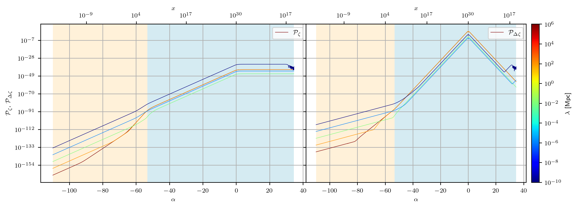
We also plot the power spectrum time evolution for \(\delta_{\rho_i}\):
Code
set_rc_params_article(ncol=2, nrows=1, aspect_ratio=aspect2c)

fig, (ax0, ax1) = plt.subplots(ncols=2, nrows=1, sharey=True)
fig.subplots_adjust(hspace=0.0, wspace=0.0)

for k, power_spectra in zip(k_values, power_spectra_list):
    lambda_com = 1.0 / k
    color = cmap(norm(lambda_com))

    ax0.plot(
        alpha_pk_a,
        k**3 * RH_Mpc**3 * power_spectra["delta_rho1"],
        lw=lw,
        linestyle="solid",
        color=color,
        label=r"$\mathcal{P}_{\delta_{\rho 1}}$" if k == k_values[0] else None,
    )
    ax1.plot(
        alpha_pk_a,
        k**3 * RH_Mpc**3 * power_spectra["delta_rho2"],
        lw=lw,
        linestyle="dashed",
        color=color,
        label=r"$\mathcal{P}_{\delta_{\rho 2}}$" if k == k_values[0] else None,
    )

ax0.set_ylabel(r"$\mathcal{P}_{\delta_{\rho i}}$")

# Shaded dominance regions
for ax in (ax0, ax1):
    ax.axvspan(alpha_pk_ini, alpha_eq, **md)
    ax.axvspan(alpha_eq, alpha_pk_end, **rd)
    ax.set_yscale("log")
    ax.legend()
    format_alpha_xaxis(ax, cosmo_rw)
    ax.set_xlabel(r"$\alpha$")
    ax.grid()


# Colorbar for k
cbar = fig.colorbar(sm, ax=(ax0, ax1), pad=0.02)
cbar.set_label(r"$\lambda$ [Mpc]")

fig.savefig(os.path.join(fig_dir, "delta_rho_power_spectrum.pdf"), bbox_inches="tight")

fig.set_size_inches(12, 12 * aspect2c)
plt.show()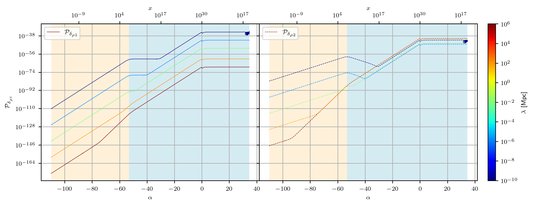
We also plot the power spectrum time evolution for \(\Delta\delta_{\zeta_i}\):
Code
set_rc_params_article(ncol=2, nrows=1, aspect_ratio=aspect2c)

fig, (ax0, ax1) = plt.subplots(ncols=2, nrows=1, sharey=True)
fig.subplots_adjust(hspace=0.0, wspace=0.0)

for k, power_spectra in zip(k_values, power_spectra_list):
    lambda_com = 1.0 / k
    color = cmap(norm(lambda_com))

    ax0.plot(
        alpha_pk_a,
        k**3 * RH_Mpc**3 * power_spectra["diff_delta_rho1"],
        lw=lw,
        linestyle="solid",
        color=color,
        label=r"$\mathcal{P}_{\Delta \delta_{\rho 1}}$" if k == k_values[0] else None,
    )
    ax1.plot(
        alpha_pk_a,
        k**3 * RH_Mpc**3 * power_spectra["diff_delta_rho2"],
        lw=lw,
        linestyle="dashed",
        color=color,
        label=r"$\mathcal{P}_{\Delta \delta_{\rho 2}}$" if k == k_values[0] else None,
    )

ax0.set_ylabel(r"$\mathcal{P}_{\Delta \delta_{\rho i}}$")

# Shaded dominance regions
for ax in (ax0, ax1):
    ax.axvspan(alpha_pk_ini, alpha_eq, **md)
    ax.axvspan(alpha_eq, alpha_pk_end, **rd)
    ax.set_yscale("log")
    ax.legend()
    format_alpha_xaxis(ax, cosmo_rw)
    ax.set_xlabel(r"$\alpha$")
    ax.grid()

# Colorbar for k
cbar = fig.colorbar(sm, ax=(ax0, ax1), pad=0.02)
cbar.set_label(r"$\lambda$ [Mpc]")

fig.savefig(
    os.path.join(fig_dir, "diff_delta_rho_power_spectrum.pdf"), bbox_inches="tight"
)

fig.set_size_inches(12, 12 * aspect2c)
plt.show()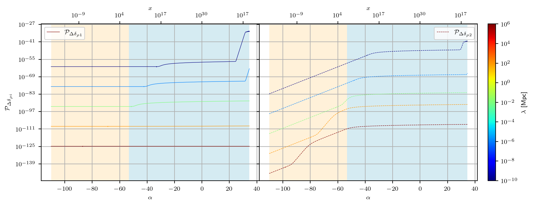
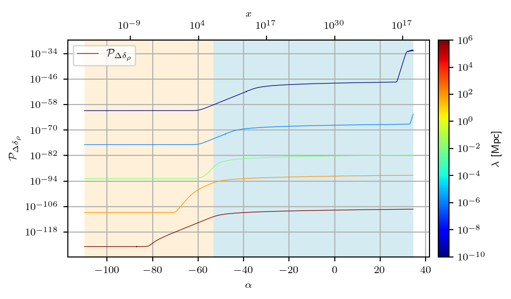
We also plot the power spectrum time evolution for the total \(\delta_{\rho}\):
Code
set_rc_params_article(ncol=1, nrows=1, aspect_ratio=0.5)

fig, ax = plt.subplots()

for k, power_spectra in zip(k_values, power_spectra_list):
    lambda_com = 1.0 / k
    color = cmap(norm(lambda_com))

    ax.plot(
        alpha_pk_a,
        k**3 * RH_Mpc**3 * power_spectra["delta_rho"],
        lw=lw,
        linestyle="solid",
        color=color,
        label=r"$\mathcal{P}_{\delta_{\rho}}$" if k == k_values[0] else None,
    )
ax.set_ylabel(r"$\mathcal{P}_{\delta_{\rho}}$")

# Shaded dominance regions
ax.axvspan(alpha_pk_ini, alpha_eq, **md)
ax.axvspan(alpha_eq, alpha_pk_end, **rd)
ax.set_yscale("log")
ax.legend()
format_alpha_xaxis(ax, cosmo_rw)
ax.set_xlabel(r"$\alpha$")
ax.grid()

# Colorbar for k
cbar = fig.colorbar(sm, ax=ax, pad=0.02)
cbar.set_label(r"$\lambda$ [Mpc]")

fig.savefig(
    os.path.join(fig_dir, "full_delta_rho_power_spectrum.pdf"), bbox_inches="tight"
)

fig.set_size_inches(6, 3)
plt.show()

fig, ax = plt.subplots()

for k, power_spectra in zip(k_values, power_spectra_list):
    lambda_com = 1.0 / k
    color = cmap(norm(lambda_com))

    ax.plot(
        alpha_pk_a,
        k**3 * RH_Mpc**3 * power_spectra["diff_delta_rho"],
        lw=lw,
        linestyle="solid",
        color=color,
        label=r"$\mathcal{P}_{\Delta \delta_{\rho}}$" if k == k_values[0] else None,
    )
ax.set_ylabel(r"$\mathcal{P}_{\Delta \delta_{\rho}}$")

# Shaded dominance regions
ax.axvspan(alpha_pk_ini, alpha_eq, **md)
ax.axvspan(alpha_eq, alpha_pk_end, **rd)
ax.set_yscale("log")
ax.legend()
format_alpha_xaxis(ax, cosmo_rw)
ax.set_xlabel(r"$\alpha$")
ax.grid()

# Colorbar for k
cbar = fig.colorbar(sm, ax=ax, pad=0.02)
cbar.set_label(r"$\lambda$ [Mpc]")

fig.savefig(
    os.path.join(fig_dir, "full_diff_delta_rho_power_spectrum.pdf"), bbox_inches="tight"
)

fig.set_size_inches(6, 3)
plt.show()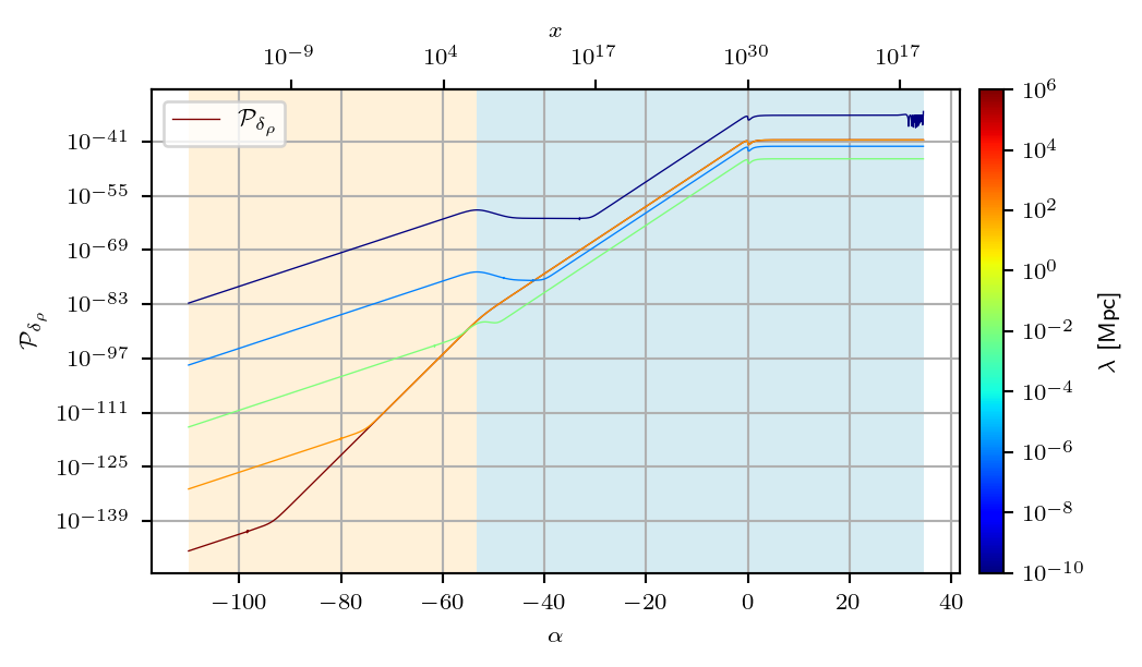
Computing Power Spectra
Now that we have seen the evolution of the adiabatic perturbations and their power spectra, we can compute the power spectra for the observables of interest. The HIPertTwoFluids object has a method called compute_power_spectra that computes the power spectra for all perturbation components, such as matter and radiation. We can use this method to compute the power spectra for the observables of interest.
pert = Nc.HIPertTwoFluids.new()
pert.props.reltol = reltol
pert.set_initial_time(alpha_ini_integ)
pert.set_final_time(alpha_end_integ)
pert.set_wkb_reltol(1.0e-3)

observables = [
    (Nc.HIPertITwoFluidsObs.ZETA, "zeta"),
    (Nc.HIPertITwoFluidsObs.ZETA_DIFF, "dzeta"),
    (Nc.HIPertITwoFluidsObs.DELTA_TOT, "delta_rho"),
    (Nc.HIPertITwoFluidsObs.DELTA_DIFF, "diff_delta_rho"),
    (Nc.HIPertITwoFluidsObs.FKU_R, "fku_r"),
    (Nc.HIPertITwoFluidsObs.FKU_W, "fku_w"),
    (Nc.HIPertITwoFluidsObs.DELTA_R, "delta_r"),
    (Nc.HIPertITwoFluidsObs.DELTA_W, "delta_w"),
    (Nc.HIPertITwoFluidsObs.PZETA, "pzeta"),
]
alpha_a = [0.01, alpha_pk_end]

# Open the log file with line buffering
with open("spectrum_progress.log", "w", buffering=1) as f:
    # Create tqdm progress bar writing to the file
    progress_bar = tqdm(total=len(k_for_pk_a), file=f, ncols=80)

    def progress_callback(step: int, _: int) -> None:
        # Update the progress bar
        progress_bar.update(1)
        progress_bar.refresh()
        f.flush()

    # Run your computation with the callback
    s_interp_a = pert.compute_spectra(
        cosmo_rw, alpha_a, k_for_pk_a * RH_Mpc, progress_callback
    )

    progress_bar.close()

power_spectra0_k = {
    f"{name}{mode_str}": np.abs(
        [
            s_interp_a[0].eval(cosmo_rw, k * RH_Mpc).eval_obs(mode, obs, obs)
            for k in k_for_plot_a
        ]
    )
    for obs, name in observables
    for mode, mode_str in [
        (Nc.HIPertITwoFluidsObsMode.ONE, "1"),
        (Nc.HIPertITwoFluidsObsMode.TWO, "2"),
        (Nc.HIPertITwoFluidsObsMode.BOTH, ""),
    ]
}

power_spectra1_k = {
    f"{name}{mode_str}": np.abs(
        [
            s_interp_a[1].eval(cosmo_rw, k * RH_Mpc).eval_obs(mode, obs, obs)
            for k in k_for_plot_a
        ]
    )
    for obs, name in observables
    for mode, mode_str in [
        (Nc.HIPertITwoFluidsObsMode.ONE, "1"),
        (Nc.HIPertITwoFluidsObsMode.TWO, "2"),
        (Nc.HIPertITwoFluidsObsMode.BOTH, ""),
    ]
}
power_spectra_k_a = [power_spectra0_k, power_spectra1_k]
Plotting the Power Spectra
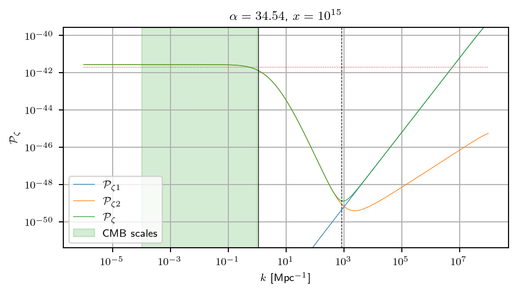
Now we can plot the power spectra for the observables of interest. We will plot the power spectra for \(\zeta\), \(\Delta\zeta\).
Code
k_pivot = 1.0
k_S_2 = k_pivot / (
    c2 * Nc.HIPertITwoFluids.eom_eval(cosmo_rw, alpha_S, k_pivot).Fnu * RH_Mpc
)
k_cross1 = k_pivot / (
    c1 * Nc.HIPertITwoFluids.eom_eval(cosmo_rw, alpha_eq, k_pivot).Fnu * RH_Mpc
)
k_cross2 = k_pivot / (
    c2 * Nc.HIPertITwoFluids.eom_eval(cosmo_rw, alpha_eq, k_pivot).Fnu * RH_Mpc
)

set_rc_params_article(ncol=1, nrows=1, aspect_ratio=0.5)

text_a = []

for i, (alpha, power_spectra_k) in enumerate(zip(alpha_a, power_spectra_k_a)):
    fig, ax = plt.subplots()

    P_zeta1_k = k_for_plot_a**3 * RH_Mpc**3 * power_spectra_k["zeta1"]
    P_zeta2_k = k_for_plot_a**3 * RH_Mpc**3 * power_spectra_k["zeta2"]
    P_zeta_k = k_for_plot_a**3 * RH_Mpc**3 * power_spectra_k["zeta"]

    ax.plot(
        k_for_plot_a,
        P_zeta1_k,
        lw=lw,
        linestyle="solid",
        label=r"$\mathcal{P}_{\zeta 1}$",
    )
    ax.plot(
        k_for_plot_a,
        P_zeta2_k,
        lw=lw,
        linestyle="solid",
        label=r"$\mathcal{P}_{\zeta 2}$",
    )
    ax.plot(
        k_for_plot_a,
        P_zeta_k,
        lw=lw,
        linestyle="solid",
        label=r"$\mathcal{P}_{\zeta}$",
    )

    AP_zeta_k = large_scale_P_zeta(k_for_plot_a * RH_Mpc)

    ax.plot(k_for_plot_a, AP_zeta_k, lw=lw, linestyle="dotted")

    ax.axvline(k_S_2, linestyle="solid", lw=lw, color="k")
    ax.axvline(k_cross2, linestyle="dashed", lw=lw, color="k")

    # Highlight the CMB-scales interval: 10^-4 < k < 10^0 Mpc^-1
    ax.axvspan(1.0e-4, 1.0e0, alpha=0.2, color="tab:green", label="CMB scales")

    ax.set_ylabel(r"$\mathcal{P}_{\zeta}$")
    ax.set_xlabel(r"$k$ [Mpc$^{-1}$]")

    x_latex = latex_float(cosmo_rw.x_alpha(alpha), precision=4)
    ax.set_title(f"$\\alpha={alpha:.2f}$, $x = {x_latex}$")
    ax.legend()
    ax.set_xscale("log")
    ax.set_yscale("log")
    ax.grid()

    ax.set_ylim(np.min(P_zeta2_k) * 1.0e-2, np.max(P_zeta2_k) * 1.0e2)

    fig.savefig(
        os.path.join(fig_dir, f"zeta_power_spectrum{i}_k.pdf"), bbox_inches="tight"
    )

    fig.set_size_inches(6, 3)
    plt.show()

    text_a.append(
        f"Ratio of power spectrum to large-scale power spectrum "
        f"approximation:\n {P_zeta1_k[0] / AP_zeta_k[0]} {P_zeta2_k[0] / AP_zeta_k[0]}"
    )

for text in text_a:
    print(text)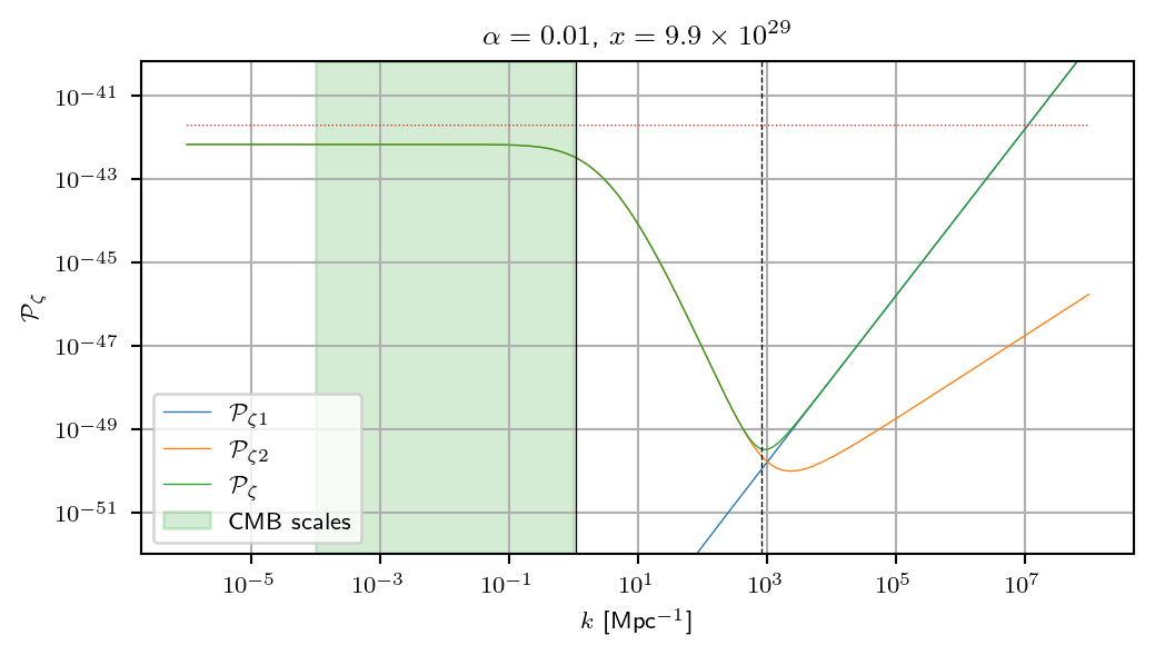
Ratio of power spectrum to large-scale power spectrum approximation:
 2.0743298150997743e-29 0.34696993344132915
Ratio of power spectrum to large-scale power spectrum approximation:
8.277611948391812e-29 1.3845834624343627Now considering a CMB-like interval (\(10^{-4} < k < 10^{0}\) Mpc\(^{-1}\)), we see that the power spectrum is dominated by the large-scale approximation together with the small-scale suppression of power. To characterize this behavior more precisely, we fit polynomials in this interval to obtain an effective spectral index. Higher-order polynomial fits additionally provide effective running and running-of-the-running parameters describing the spectrum within the CMB scales.
power_spectra_k = power_spectra_k_a[1]
k_for_cmb_constraint = k_for_plot_a < 1.0
k_for_cmb = k_for_plot_a[k_for_cmb_constraint]
# Using same pivot scale as Planck 2018 k0 = 0.05 Mpc^-1
lnk_for_cmb = np.log(k_for_plot_a[k_for_cmb_constraint] / 0.05)
ln_zeta_cmb = np.log(
    RH_Mpc**3 * k_for_cmb**3 * power_spectra_k["zeta"][k_for_cmb_constraint]
)

# Linear fit (spectral index only)
fit_lin = np.polyfit(lnk_for_cmb, ln_zeta_cmb, deg=1)
ns_lin = fit_lin[-2] + 1.0

# Quadratic fit (spectral index + running)
fit_quad = np.polyfit(lnk_for_cmb, ln_zeta_cmb, deg=2)
ns_quad = fit_quad[-2] + 1.0
alpha_s = fit_quad[-3] * 2.0

# Cubic fit (spectral index + running + running of running)
fit_cubic = np.polyfit(lnk_for_cmb, ln_zeta_cmb, deg=3)
ns_cubic = fit_cubic[-2] + 1.0
alpha_s_cubic = fit_cubic[-3] * 2.0
beta_s = fit_cubic[-4] * 6.0

# Report
report = f"""
### Fit to the power spectrum in the CMB-scales interval

**Linear fit (constant spectral index):**

- Effective spectral index: {ns_lin:.4f}

**Quadratic fit (including running):**

- Effective spectral index: {ns_quad:.4f}
- Running parameter: {alpha_s:.4f}

**Cubic fit (including running of running):**

- Effective spectral index: {ns_cubic:.4f}
- Running parameter: {alpha_s_cubic:.4f}
- Running of the running: {beta_s:.4f}
"""
display(Markdown(report))
Fit to the power spectrum in the CMB-scales interval
Linear fit (constant spectral index):
- Effective spectral index: 0.9851
Quadratic fit (including running):
- Effective spectral index: 0.9514
- Running parameter: -0.0086
Cubic fit (including running of running):
- Effective spectral index: 0.9334
- Running parameter: -0.0331
- Running of the running: -0.0063
Now we can plot this CMB-like section of the power spectrum and overplot the linear, quadratic, and cubic fits used to extract an effective spectral index, running, and running of the running.
Code
set_rc_params_article(ncol=1, nrows=1, aspect_ratio=0.5)

power_spectra_k = power_spectra_k_a[1]
fig, ax = plt.subplots()

P_zeta_k = k_for_cmb**3 * RH_Mpc**3 * power_spectra_k["zeta"][k_for_cmb_constraint]
P_zeta_lin_k = np.exp(fit_lin[0] * lnk_for_cmb + fit_lin[1])
P_zeta_quad_k = np.exp(
    fit_quad[0] * lnk_for_cmb**2 + fit_quad[1] * lnk_for_cmb + fit_quad[2]
)
P_zeta_cubic_k = np.exp(
    fit_cubic[0] * lnk_for_cmb**3
    + fit_cubic[1] * lnk_for_cmb**2
    + fit_cubic[2] * lnk_for_cmb
    + fit_cubic[3]
)

ax.plot(k_for_cmb, P_zeta_k, lw=lw, linestyle="solid", label=r"$\mathcal{P}_{\zeta}$")
ax.plot(
    k_for_cmb,
    P_zeta_lin_k,
    lw=lw,
    linestyle="dashed",
    label=r"$\mathcal{P}_{\zeta}$ (linear fit)",
)
ax.plot(
    k_for_cmb,
    P_zeta_quad_k,
    lw=lw,
    linestyle="dotted",
    label=r"$\mathcal{P}_{\zeta}$ (quadratic fit)",
)
ax.plot(
    k_for_cmb,
    P_zeta_cubic_k,
    lw=lw,
    linestyle=(0, (3, 1, 1, 1)),
    label=r"$\mathcal{P}_{\zeta}$ (cubic fit)",
)

ax.set_ylabel(r"$\mathcal{P}_{\zeta}$")
ax.set_xlabel(r"$k$ [Mpc$^{-1}$]")

ax.legend()
ax.set_xscale("log")
# ax.set_yscale("log")
ax.grid()

fig.savefig(os.path.join(fig_dir, "zeta_power_spectrum_cmb_k.pdf"), bbox_inches="tight")

fig.set_size_inches(6, 3)
plt.show()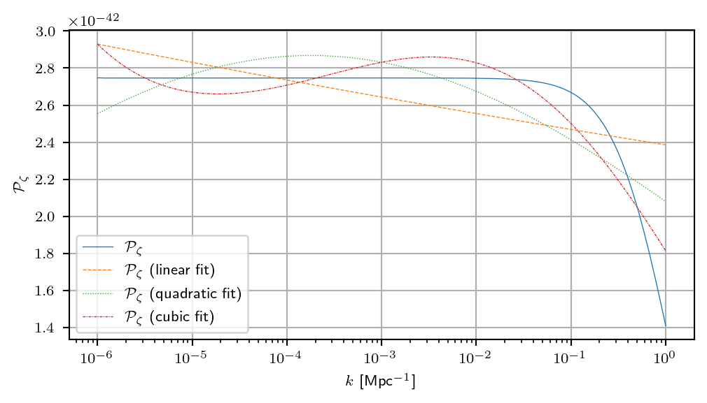
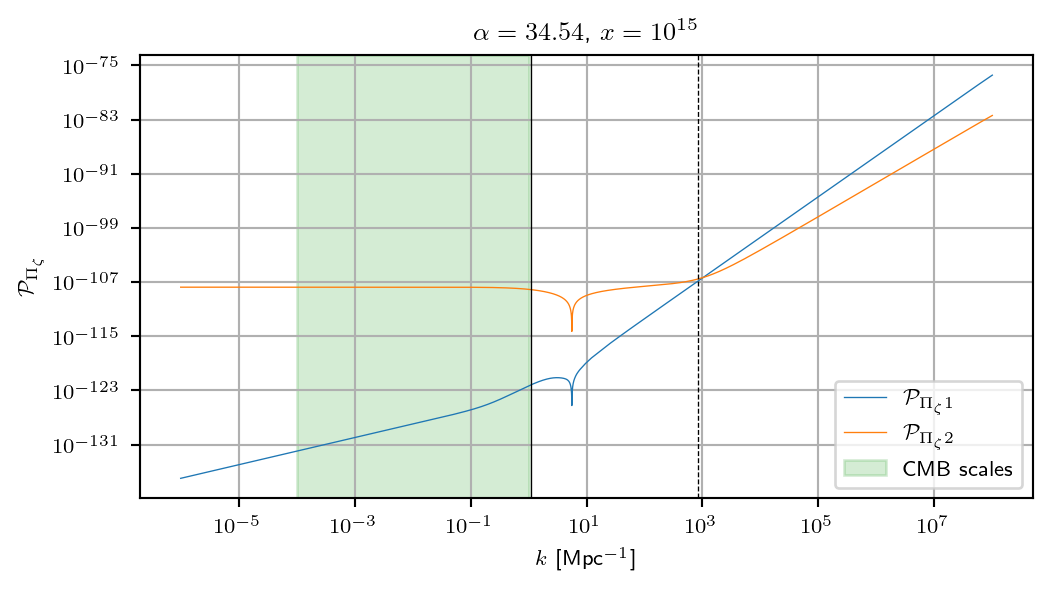
Next we plot the power spectra for \(\Pi_\zeta\) and \(\Delta\Pi_\zeta\):
Code
set_rc_params_article(ncol=1, nrows=1, aspect_ratio=0.5)

for i, (alpha, power_spectra_k) in enumerate(zip(alpha_a, power_spectra_k_a)):
    fig, ax = plt.subplots()

    P_pzeta1_k = k_for_plot_a**3 * RH_Mpc**3 * power_spectra_k["pzeta1"]
    P_pzeta2_k = k_for_plot_a**3 * RH_Mpc**3 * power_spectra_k["pzeta2"]

    ax.plot(
        k_for_plot_a,
        P_pzeta1_k,
        lw=lw,
        linestyle="solid",
        label=r"$\mathcal{P}_{\Pi_\zeta 1}$",
    )
    ax.plot(
        k_for_plot_a,
        P_pzeta2_k,
        lw=lw,
        linestyle="solid",
        label=r"$\mathcal{P}_{\Pi_\zeta 2}$",
    )

    ax.axvline(k_S_2, linestyle="solid", lw=lw, color="k")
    ax.axvline(k_cross2, linestyle="dashed", lw=lw, color="k")

    # Highlight the CMB-scales interval: 10^-4 < k < 10^0 Mpc^-1
    ax.axvspan(1.0e-4, 1.0e0, alpha=0.2, color="tab:green", label="CMB scales")

    ax.set_ylabel(r"$\mathcal{P}_{\Pi_\zeta}$")
    ax.set_xlabel(r"$k$ [Mpc$^{-1}$]")

    x_latex = latex_float(cosmo_rw.x_alpha(alpha), precision=4)
    ax.set_title(f"$\\alpha={alpha:.2f}$, $x = {x_latex}$")
    ax.legend()
    ax.set_xscale("log")
    ax.set_yscale("log")
    ax.grid()

    fig.savefig(
        os.path.join(fig_dir, f"Pzeta_power_spectrum{i}_k.pdf"), bbox_inches="tight"
    )

    fig.set_size_inches(6, 3)
    plt.show()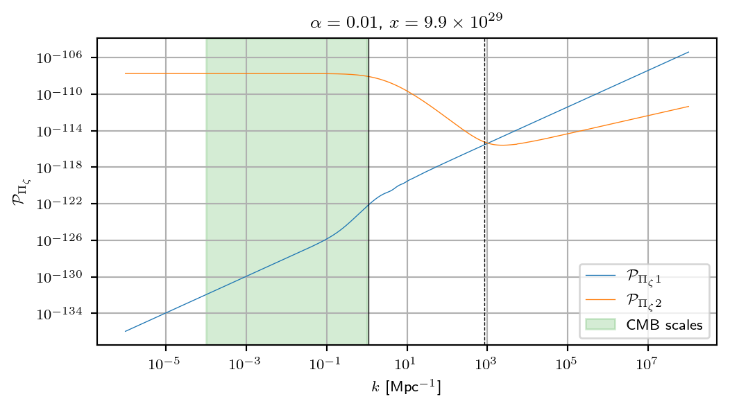
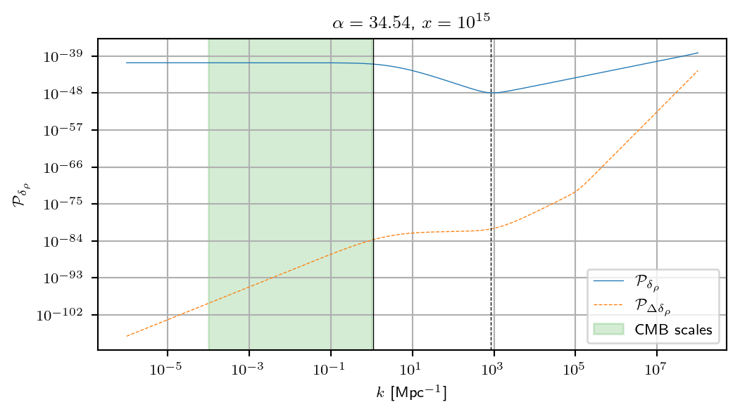
Next we plot the power spectra for \(\delta_{\rho}\) and \(\Delta\delta_{\rho}\):
Code
set_rc_params_article(ncol=1, nrows=1, aspect_ratio=0.5)

for i, (alpha, power_spectra_k) in enumerate(zip(alpha_a, power_spectra_k_a)):
    fig, ax = plt.subplots()

    ax.plot(
        k_for_plot_a,
        k_for_plot_a**3 * RH_Mpc**3 * power_spectra_k["delta_rho"],
        lw=lw,
        linestyle="solid",
        label=r"$\mathcal{P}_{\delta_{\rho}}$",
    )

    ax.plot(
        k_for_plot_a,
        k_for_plot_a**3 * RH_Mpc**3 * power_spectra_k["diff_delta_rho"],
        lw=lw,
        linestyle="dashed",
        label=r"$\mathcal{P}_{\Delta \delta_{\rho}}$",
    )

    ax.axvline(k_S_2, linestyle="solid", lw=lw, color="k")
    ax.axvline(k_cross2, linestyle="dashed", lw=lw, color="k")

    # Highlight the CMB-scales interval: 10^-4 < k < 10^0 Mpc^-1
    ax.axvspan(1.0e-4, 1.0e0, alpha=0.2, color="tab:green", label="CMB scales")

    ax.set_ylabel(r"$\mathcal{P}_{\delta_{\rho}}$")
    ax.set_xlabel(r"$k$ [Mpc$^{-1}$]")

    x_latex = latex_float(cosmo_rw.x_alpha(alpha), precision=4)
    ax.set_title(f"$\\alpha={alpha:.2f}$, $x = {x_latex}$")
    ax.legend()
    ax.set_xscale("log")
    ax.set_yscale("log")
    ax.grid()

    fig.savefig(
        os.path.join(fig_dir, f"delta_rho_power_spectrum{i}_k.pdf"), bbox_inches="tight"
    )
    fig.set_size_inches(6, 3)
    plt.show()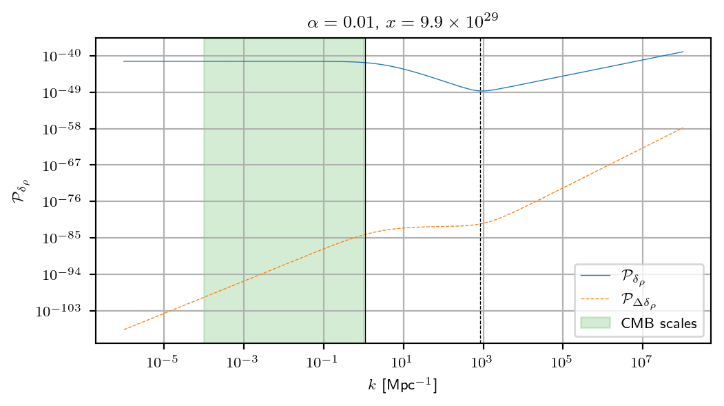
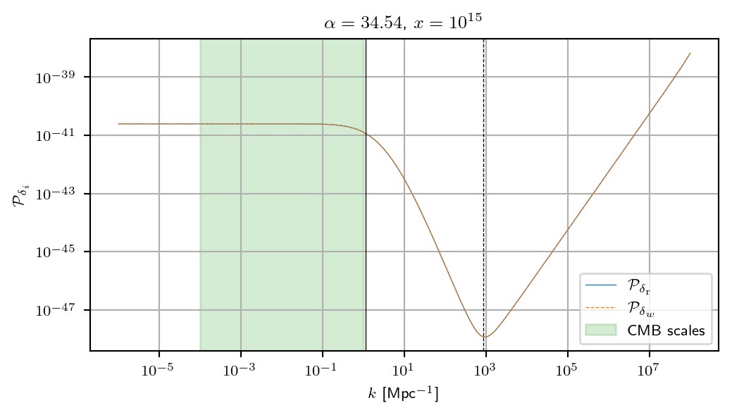
We can also plot the power spectra for the individual fluid density perturbations \(\delta_{\mathrm{r}}\) and \(\delta_{w}\):
Code
set_rc_params_article(ncol=1, nrows=1, aspect_ratio=0.5)

for i, (alpha, power_spectra_k) in enumerate(zip(alpha_a, power_spectra_k_a)):
    fig, ax = plt.subplots()

    ax.plot(
        k_for_plot_a,
        k_for_plot_a**3 * RH_Mpc**3 * power_spectra_k["delta_r"],
        lw=lw,
        linestyle="solid",
        label=r"$\mathcal{P}_{\delta_{\mathrm{r}}}$",
    )

    ax.plot(
        k_for_plot_a,
        k_for_plot_a**3 * RH_Mpc**3 * power_spectra_k["delta_w"],
        lw=lw,
        linestyle="dashed",
        label=r"$\mathcal{P}_{\delta_{w}}$",
    )

    ax.axvline(k_S_2, linestyle="solid", lw=lw, color="k")
    ax.axvline(k_cross2, linestyle="dashed", lw=lw, color="k")

    # Highlight the CMB-scales interval: 10^-4 < k < 10^0 Mpc^-1
    ax.axvspan(1.0e-4, 1.0e0, alpha=0.2, color="tab:green", label="CMB scales")

    ax.set_ylabel(r"$\mathcal{P}_{\delta_{i}}$")
    ax.set_xlabel(r"$k$ [Mpc$^{-1}$]")

    x_latex = latex_float(cosmo_rw.x_alpha(alpha), precision=4)
    ax.set_title(f"$\\alpha={alpha:.2f}$, $x = {x_latex}$")
    ax.legend()
    ax.set_xscale("log")
    ax.set_yscale("log")
    ax.grid()

    fig.savefig(
        os.path.join(fig_dir, f"delta_rw_power_spectrum{i}_k.pdf"), bbox_inches="tight"
    )
    fig.set_size_inches(6, 3)
    plt.show()
The fluid velocity potentials \(\mathcal{V}_{\mathrm{r}}\) and \(\mathcal{V}_{w}\):
Code
set_rc_params_article(ncol=2, nrows=1, aspect_ratio=aspect2c)

fig, (ax0, ax1) = plt.subplots(ncols=2, nrows=1, sharey=True)
fig.subplots_adjust(hspace=0.0, wspace=0.0)

for i, (alpha, power_spectra_k, ax) in enumerate(
    zip(alpha_a, power_spectra_k_a, [ax0, ax1])
):
    ax.plot(
        k_for_plot_a,
        k_for_plot_a**3 * RH_Mpc**3 * power_spectra_k["fku_r"],
        lw=lw,
        linestyle="solid",
        label=r"$\mathcal{P}_{\mathcal{V}_{\mathrm{r}}}$",
        alpha=0.8,
    )

    ax.plot(
        k_for_plot_a,
        k_for_plot_a**3 * RH_Mpc**3 * power_spectra_k["fku_w"],
        lw=lw,
        linestyle="dashed",
        label=r"$\mathcal{P}_{\mathcal{V}_{w}}$",
    )

    ax.axvline(k_S_2, linestyle="solid", lw=lw, color="k")
    ax.axvline(k_cross2, linestyle="dashed", lw=lw, color="k")

    # Highlight the CMB-scales interval: 10^-4 < k < 10^0 Mpc^-1
    ax.axvspan(1.0e-4, 1.0e0, alpha=0.2, color="tab:green", label="CMB scales")

    if i == 0:
        ax.set_ylabel(r"$\mathcal{P}_{\mathcal{V}_{i}}$")
    ax.set_xlabel(r"$k$ [Mpc$^{-1}$]")

    x_latex = latex_float(cosmo_rw.x_alpha(alpha), precision=4)
    ax.set_title(f"$\\alpha={alpha:.2f}$, $x = {x_latex}$")
    if i == 0:
        ax.legend()

    ax.set_xscale("log")
    ax.set_yscale("log")
    ax.grid()

fig.savefig(os.path.join(fig_dir, f"fku_rw_power_spectrum_k.pdf"), bbox_inches="tight")

fig.set_size_inches(12, 12 * aspect2c)
plt.show()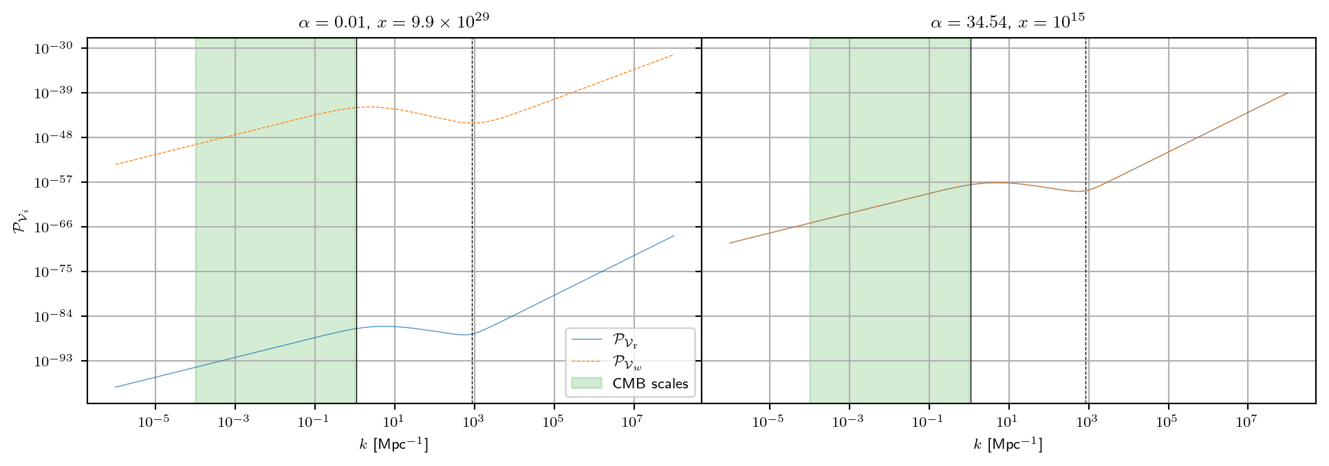
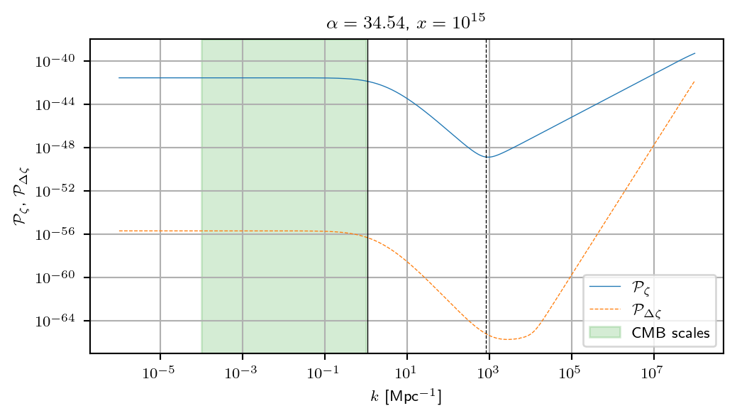
We can also plot \(\zeta\) and \(\Delta\zeta\) in the same plot to observe another source of isocurvature.
Code
set_rc_params_article(ncol=1, nrows=1, aspect_ratio=0.5)

for i, (alpha, power_spectra_k) in enumerate(zip(alpha_a, power_spectra_k_a)):
    fig, ax = plt.subplots()

    ax.plot(
        k_for_plot_a,
        k_for_plot_a**3 * RH_Mpc**3 * power_spectra_k["zeta"],
        lw=lw,
        linestyle="solid",
        label=r"$\mathcal{P}_{\zeta}$",
    )

    ax.plot(
        k_for_plot_a,
        k_for_plot_a**3 * RH_Mpc**3 * power_spectra_k["dzeta"],
        lw=lw,
        linestyle="dashed",
        label=r"$\mathcal{P}_{\Delta \zeta}$",
    )

    ax.axvline(k_S_2, linestyle="solid", lw=lw, color="k")
    ax.axvline(k_cross2, linestyle="dashed", lw=lw, color="k")

    # Highlight the CMB-scales interval: 10^-4 < k < 10^0 Mpc^-1
    ax.axvspan(1.0e-4, 1.0e0, alpha=0.2, color="tab:green", label="CMB scales")

    ax.set_ylabel(r"$\mathcal{P}_{\zeta}$, $\mathcal{P}_{\Delta \zeta}$")
    ax.set_xlabel(r"$k$ [Mpc$^{-1}$]")

    x_latex = latex_float(cosmo_rw.x_alpha(alpha), precision=4)
    ax.set_title(f"$\\alpha={alpha:.2f}$, $x = {x_latex}$")
    ax.legend()
    ax.set_xscale("log")
    ax.set_yscale("log")
    ax.grid()

    fig.savefig(
        os.path.join(fig_dir, f"zeta_dzeta_power_spectrum{i}_k.pdf"),
        bbox_inches="tight",
    )
    fig.set_size_inches(6, 3)
    plt.show()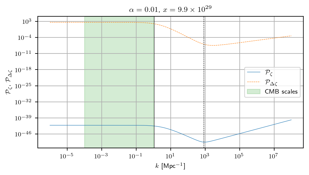
Tensor power spectrum
Now we can also compute the tensor power spectrum.
pgw = Nc.HIPertGW.new()

pgw.set_initial_condition_type(Ncm.CSQ1DInitialStateType.ADIABATIC4)
pgw.set_ti(alpha_pk_ini)
pgw.set_tf(alpha_pk_end)
pgw.set_vacuum_max_time(-1.0e-1)
pgw.set_vacuum_reltol(1.0e-8)
Ncm.CSQ1D.set_reltol(pgw, 1.0e-10)

gw_pk_evol = []

for k in k_values:
    pgw.set_k(k * RH_Mpc)
    pgw.prepare(cosmo_rw)

    pk = np.array([pgw.eval_powspec_at(cosmo_rw, alpha) for alpha in alpha_pk_a])
    gw_pk_evol.append(pk)

gw_pk_k = []

for alpha in alpha_a:
    gw_pk_k.append(pgw.eval_powspec(cosmo_rw, alpha, k_for_pk_a * RH_Mpc))
We can plot the tensor power spectrum evolution for each mode:
Code
set_rc_params_article(ncol=1, nrows=1, aspect_ratio=0.5)
fig, ax = plt.subplots()

for k, gw_pk in zip(k_values, gw_pk_evol):
    lambda_com = 1.0 / k
    color = cmap(norm(lambda_com))

    ax.plot(
        alpha_pk_a,
        k**3 * RH_Mpc**3 * gw_pk,
        lw=lw,
        linestyle="solid",
        color=color,
    )

format_alpha_xaxis(ax, cosmo_rw)
ax.set_xlabel(r"$\alpha$")
ax.set_ylabel(r"$\mathcal{P}_{h}$")
ax.set_yscale("log")
ax.grid()

# Colorbar for k
cbar = fig.colorbar(sm, ax=ax, pad=0.02)
cbar.set_label(r"$\lambda$ [Mpc]")

fig.savefig(os.path.join(fig_dir, f"tensor_pw_evol.pdf"), bbox_inches="tight")
fig.set_size_inches(6, 3)
plt.show()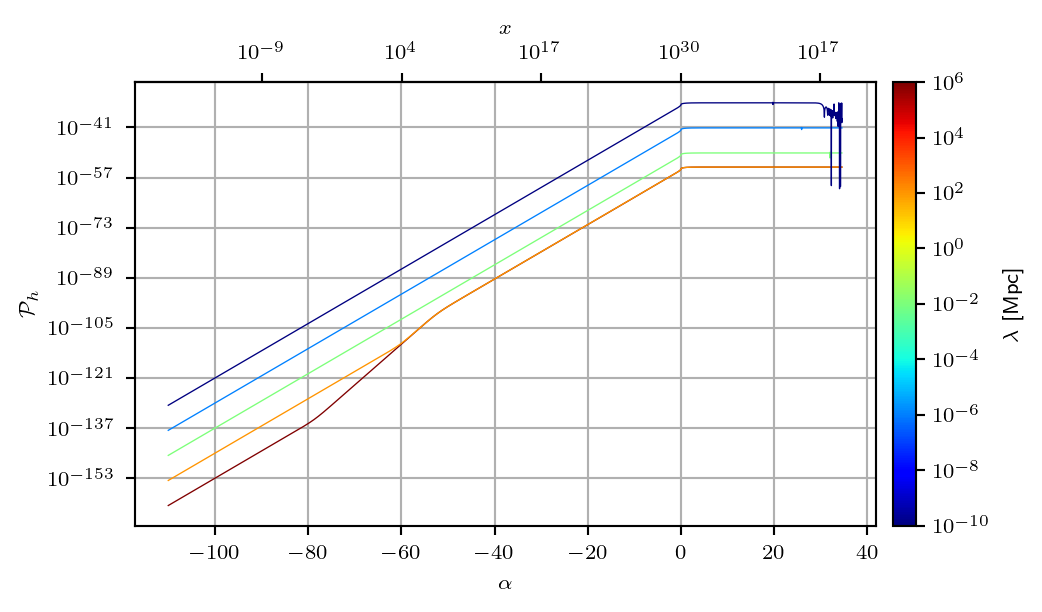
We can also plot it at the final time:
Code
set_rc_params_article(ncol=1, nrows=1, aspect_ratio=0.5)

for i, alpha in enumerate(alpha_a):
    fig, ax = plt.subplots()

    gw_pk_k_a = np.array([gw_pk_k[i].eval(k * RH_Mpc) for k in k_for_plot_a])

    ax.plot(
        k_for_plot_a,
        k_for_plot_a**3 * RH_Mpc**3 * gw_pk_k_a,
        lw=lw,
        linestyle="solid",
        label=r"$\mathcal{P}_{h}$",
    )

    # Highlight the CMB-scales interval: 10^-4 < k < 10^0 Mpc^-1
    ax.axvspan(1.0e-4, 1.0e0, alpha=0.2, color="tab:green", label="CMB scales")

    ax.set_ylabel(r"$\mathcal{P}_{h}$")
    ax.set_xlabel(r"$k$ [Mpc$^{-1}$]")

    x_latex = latex_float(cosmo_rw.x_alpha(alpha), precision=4)
    ax.set_title(f"$\\alpha={alpha:.2f}$, $x = {x_latex}$")
    ax.legend()
    ax.set_xscale("log")
    ax.set_yscale("log")
    ax.grid()

    fig.savefig(os.path.join(fig_dir, f"tensor_pw{i}_k.pdf"), bbox_inches="tight")
    fig.set_size_inches(6, 3)
plt.show()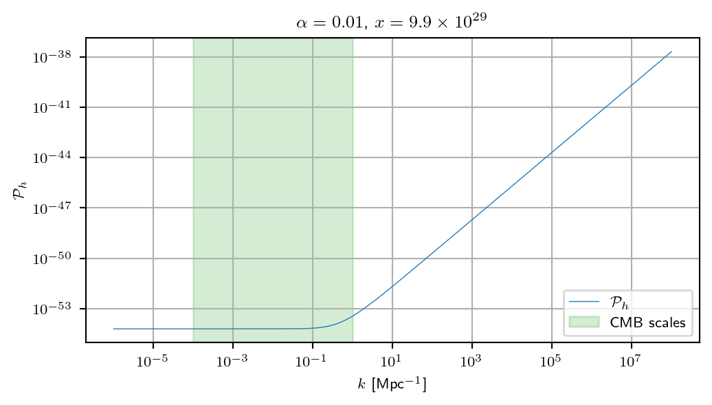

Tensor-to-scalar ratio
The tensor-to-scalar ratio \(r\) is a key observable in cosmology, defined as the ratio of the tensor power spectrum (accounting for two polarization states) to the total scalar (curvature) power spectrum:
\[ r(k) = \frac{\mathcal{P}_h(k)}{\mathcal{P}_\zeta(k)} \]
This ratio provides important constraints on the underlying physics of the early universe. In standard slow-roll inflation, \(r\) is directly related to the energy scale of inflation.
# Compute tensor-to-scalar ratio at selected times
tensor_to_scalar_ratio = []
for i, alpha in enumerate(alpha_a):
gw_pk_k_a = np.array([gw_pk_k[i].eval(k * RH_Mpc) for k in k_for_plot_a])
zeta_pk_k_a = power_spectra_k_a[i]["zeta"]
# r = 2*P_h / P_zeta (factor of 2 for two polarizations)
r_k = 2.0 * gw_pk_k_a / zeta_pk_k_a
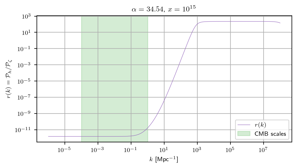
tensor_to_scalar_ratio.append(r_k)We can plot the tensor-to-scalar ratio as a function of wavenumber:
Code
set_rc_params_article(ncol=1, nrows=1, aspect_ratio=0.5)

for i, alpha in enumerate(alpha_a):
    fig, ax = plt.subplots()

    ax.plot(
        k_for_plot_a,
        tensor_to_scalar_ratio[i],
        lw=lw,
        linestyle="solid",
        label=r"$r(k)$",
        color="tab:purple",
    )

    # Highlight the CMB-scales interval: 10^-4 < k < 10^0 Mpc^-1
    ax.axvspan(1.0e-4, 1.0e0, alpha=0.2, color="tab:green", label="CMB scales")

    ax.set_ylabel(r"$r(k) = \mathcal{P}_h / \mathcal{P}_\zeta$")
    ax.set_xlabel(r"$k$ [Mpc$^{-1}$]")

    x_latex = latex_float(cosmo_rw.x_alpha(alpha), precision=4)
    ax.set_title(f"$\\alpha={alpha:.2f}$, $x = {x_latex}$")
    ax.legend()
    ax.set_xscale("log")
    ax.set_yscale("log")
    ax.grid()

    fig.savefig(
        os.path.join(fig_dir, f"tensor_to_scalar_ratio{i}_k.pdf"), bbox_inches="tight"
    )
    fig.set_size_inches(6, 3)
plt.show()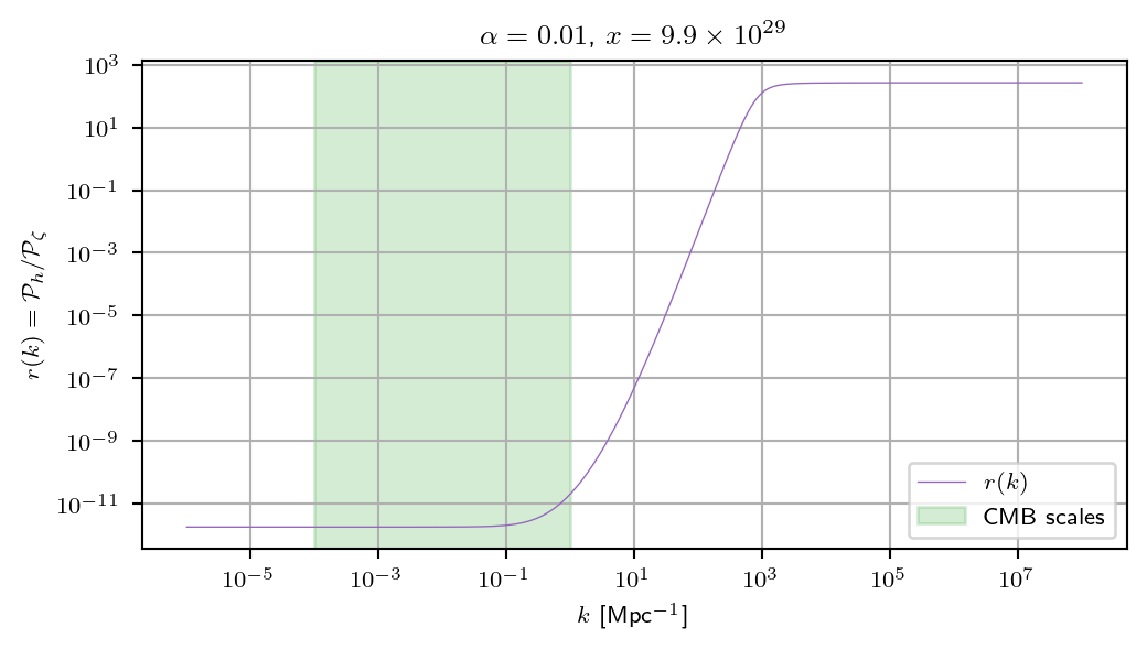
We can also compute the mean tensor-to-scalar ratio in the CMB-scales interval (\(10^{-4} < k < 10^0\) Mpc\(^{-1}\)):
# Compute mean r in CMB scales
k_cmb_mask = (k_for_plot_a >= 1.0e-4) & (k_for_plot_a <= 1.0e0)

for i, alpha in enumerate(alpha_a):
    r_cmb_mean = np.mean(tensor_to_scalar_ratio[i][k_cmb_mask])
    x_latex = latex_float(cosmo_rw.x_alpha(alpha), precision=4)
    print(f"α = {alpha:.2f}, x = {x_latex}: mean r in CMB scales = {r_cmb_mean:.4e}")
α = 0.01, x = 9.9 \times 10^{29}: mean r in CMB scales = 2.8118e-12
α = 34.54, x = 10^{15}: mean r in CMB scales = 2.3728e-12Preparing the fiducial power spectrum
Testing the calibrated model
The HIPrimTwoFluids model includes a pre-calibrated version that loads normalization data from a binary file. This calibration includes a 2D spline for the normalized power spectrum and a 1D spline (Pk0) that describes how the normalization at \(k_{\min}\) scales with the equation-of-state parameter \(w\).
We can load the calibrated model and verify the expected scaling relationship: \(\ln P_{k_0} \propto -\frac{5}{2} \ln w\).
# Load the calibration data directly from the binary file
ser = Ncm.Serialize.new(Ncm.SerializeOpt.CLEAN_DUP)
default_calib_file = Ncm.cfg_get_data_filename("hiprim_2f_var.bin", True)
calib_dict = ser.dict_str_from_binfile(default_calib_file)
Pk0 = calib_dict.get("Pk0")
assert isinstance(Pk0, Ncm.Spline)
Pk0.prepare()

# Define a range of w values for testing
w_range = np.geomspace(1.0e-9, 1.0e-2, 100)
lnw_range = np.log(w_range)

# Evaluate the Pk0 spline at these w values
lnPk0_values = np.array([Pk0.eval(lnw) for lnw in lnw_range])
Pk0_values = np.exp(lnPk0_values)

# Perform linear fit in log-log space to extract the scaling exponent
coeffs = np.polyfit(lnw_range, lnPk0_values, 1)
lnPk0_fit = np.polyval(coeffs, lnw_range)

print(f"Linear fit in log-log space:")
print(f"  Slope: {coeffs[0]:.6f} (expected: -2.5)")
print(f"  Intercept: {coeffs[1]:.6f}")
print(f"  Deviation from expected slope: {abs(coeffs[0] + 2.5):.6f}")
Linear fit in log-log space:
Slope: -2.523400 (expected: -2.5)
Intercept: -135.211485
Deviation from expected slope: 0.023400Now we can visualize this scaling relationship:
Code
set_rc_params_article(ncol=1, nrows=1, aspect_ratio=0.5)
fig, ax = plt.subplots()

# Plot the spline data
ax.plot(
    w_range,
    Pk0_values,
    "b-",
    linewidth=lw,
    label=r"$\bar{\mathcal{P}}(10^{-3}; w)$",
)

# Add expected slope line (slope = -2.5)
expected_slope = -2.5
lnw_ref = lnw_range[0]
lnPk0_ref = lnPk0_values[0]
lnPk0_expected = expected_slope * (lnw_range - lnw_ref) + lnPk0_ref
Pk0_expected = np.exp(lnPk0_expected)

ax.plot(
    w_range,
    Pk0_expected,
    "r--",
    linewidth=lw,
    label=f"Expected: slope={expected_slope}",
)

ax.set_xscale("log")
ax.set_yscale("log")
ax.set_xlabel(r"$w$")
ax.set_ylabel(r"$\bar{\mathcal{P}}(10^{-3}; w)$")
ax.set_title(r"Normalization $\bar{\mathcal{P}}(10^{-3}; w)$")
ax.legend(loc="best")
ax.grid(True, alpha=0.3)

plt.savefig(os.path.join(fig_dir, "pk0_scaling.pdf"), bbox_inches="tight")
fig.set_size_inches(6, 3)
plt.show()

print(f"Expected slope: {expected_slope}")
print(f"Reference point: w = {w_range[0]:.2e}, lnPk0 = {lnPk0_ref:.6f}")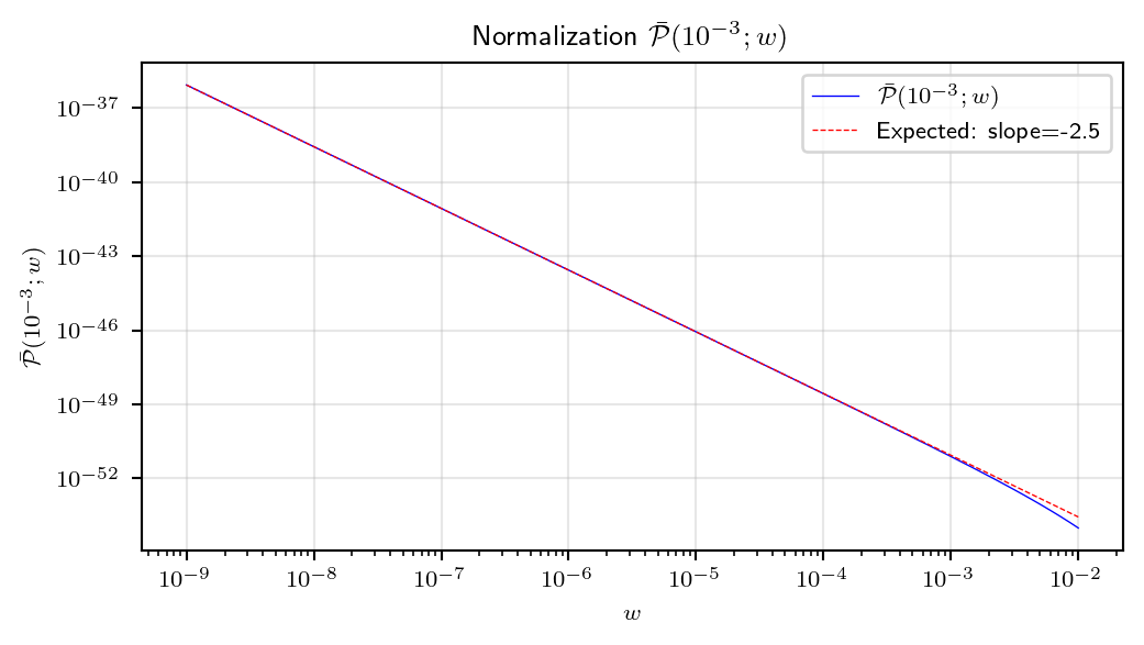
Expected slope: -2.5
Reference point: w = 1.00e-09, lnPk0 = -83.033933
We can also examine the normalized power spectrum by dividing out the expected scaling factor:
Code
# Compute the normalization factor
xb = cosmo_rw.props.xb
Omegar = cosmo_rw.props.Omegar
Omegaw = cosmo_rw.props.Omegaw
RH_planck = cosmo_rw.RH_planck()

# For each w value, compute c_w = sqrt(w) and the normalization
normalization = np.array(
    [(xb**2 * Omegaw**2) / (RH_planck**2 * Omegar * np.sqrt(w) ** 5) for w in w_range]
)

Pk0_normalized = Pk0_values / normalization

set_rc_params_article(ncol=1, nrows=1, aspect_ratio=0.5)
fig, ax = plt.subplots()

ax.plot(
    w_range,
    Pk0_normalized,
    "b-",
    linewidth=lw,
    label=r"Normalized $\bar{\mathcal{P}}(10^{-3}; w)$",
)

ax.set_xscale("log")
ax.set_xlabel(r"$w$")
ax.set_ylabel(
    r"$\bar{\mathcal{P}}(10^{-3}; w) / \left(\ell_\textsc{P}^2 x_b^2 \Omega_w^2 / (R_H^2 \Omega_r c_w^5) \right)$"
)
ax.set_title(r"Normalized power spectrum at $\kappa = 10^{-3}$")
ax.legend(loc="best")
ax.grid(True, alpha=0.3)

plt.savefig(os.path.join(fig_dir, "pk0_normalized.pdf"), bbox_inches="tight")
fig.set_size_inches(6, 3)
plt.show()

print(f"Normalized Pk0 range: [{Pk0_normalized.min():.6e}, {Pk0_normalized.max():.6e}]")
print(f"Variation: {Pk0_normalized.max() / Pk0_normalized.min():.4f}x")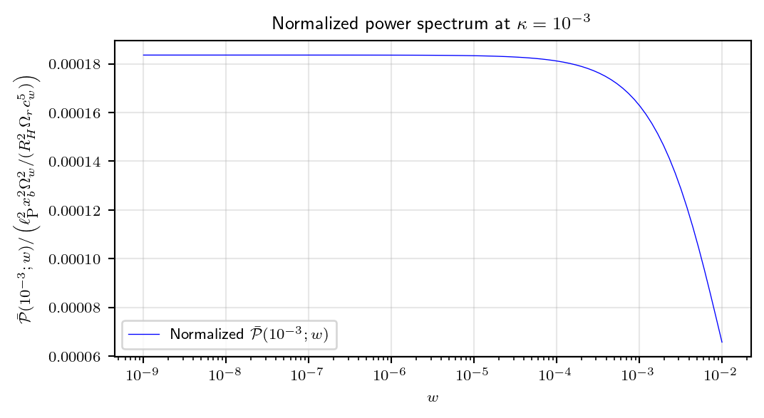
Normalized Pk0 range: [6.566102e-05, 1.836318e-04]
Variation: 2.7967x
CMB Power Spectra Comparison
Now we compute the CMB temperature angular power spectra (\(C_\ell^{TT}\)) for both the two-fluids bounce model and the standard power-law inflationary model. This comparison shows how the primordial spectrum differences propagate to observable CMB anisotropies.
We use the Boltzmann code interface (HIPertBoltzmannCBE) to compute the lensed \(C_\ell\) spectra up to \(\ell_{\rm max} = 2500\). The two models are fitted to Planck 2018 data with their respective best-fit cosmological parameters.
Code
def compute_D_ell_twofluid(lmax=2500):
    """Compute CMB TT power spectrum for two-fluids bounce model."""
    # Setup precision and Boltzmann code
    cbe_prec = Nc.CBEPrecision.new()
    cbe_prec.props.k_per_decade_primordial = 50.0
    cbe_prec.props.tight_coupling_approximation = 0

    cbe = Nc.CBE.prec_new(cbe_prec)

    Bcbe = Nc.HIPertBoltzmannCBE.full_new(cbe)
    Bcbe.set_TT_lmax(lmax)
    Bcbe.set_target_Cls(Nc.DataCMBDataType.TT)
    Bcbe.set_lensed_Cls(True)

    # Setup cosmology with two-fluids primordial spectrum
    cosmo = Nc.HICosmoDEXcdm.new()
    cosmo.cmb_params()
    reion = Nc.HIReionCamb.new()
    hiprim = Nc.HIPrimTwoFluids(use_default_calib=True)

    # Best-fit parameters for Planck 2018 with two-fluids model
    cosmo["Omegak"] = 0.0
    cosmo["H0"] = 69.5616151425007
    cosmo["omegab"] = 0.0226931446150128
    cosmo["omegac"] = 0.116422916054973
    hiprim["ln10e10ASA"] = 3.07203761177891
    hiprim["lnk0"] = -6.251936466867
    hiprim["lnw"] = -12.6152819113359
    reion["z_re"] = 8.35735404822378

    cosmo.add_submodel(reion)
    cosmo.add_submodel(hiprim)

    Bcbe.prepare(cosmo)

    # Extract TT power spectrum
    Cls = Ncm.Vector.new(lmax + 1)
    Bcbe.get_TT_Cls(Cls)

    Cls_a = np.array(Cls.dup_array())[2:]
    ell = np.arange(2, lmax + 1)

    # Convert to D_ell = ell(ell+1) C_ell / (2pi)
    Dls_a = ell * (ell + 1.0) * Cls_a / (2.0 * np.pi)

    return ell, Dls_a


def compute_D_ell_powerlaw(lmax=2500):
    """Compute CMB TT power spectrum for power-law inflationary model."""
    # Setup precision and Boltzmann code
    cbe_prec = Nc.CBEPrecision.new()
    cbe_prec.props.k_per_decade_primordial = 50.0
    cbe_prec.props.tight_coupling_approximation = 0

    cbe = Nc.CBE.prec_new(cbe_prec)

    Bcbe = Nc.HIPertBoltzmannCBE.full_new(cbe)
    Bcbe.set_TT_lmax(lmax)
    Bcbe.set_target_Cls(Nc.DataCMBDataType.TT)
    Bcbe.set_lensed_Cls(True)

    # Setup cosmology with power-law primordial spectrum
    cosmo = Nc.HICosmoDEXcdm.new()
    cosmo.cmb_params()
    reion = Nc.HIReionCamb.new()
    hiprim = Nc.HIPrimPowerLaw()

    # Best-fit parameters for Planck 2018 with power-law model
    cosmo["Omegak"] = 0.0
    cosmo["H0"] = 68.2682642143184
    cosmo["omegab"] = 0.0223445767610612
    cosmo["omegac"] = 0.1189257178946
    hiprim["ln10e10ASA"] = 3.04632994161073
    hiprim["n_SA"] = 0.967382455314431
    reion["z_re"] = 7.79677265563444

    cosmo.add_submodel(reion)
    cosmo.add_submodel(hiprim)

    Bcbe.prepare(cosmo)

    # Extract TT power spectrum
    Cls = Ncm.Vector.new(lmax + 1)
    Bcbe.get_TT_Cls(Cls)

    Cls_a = np.array(Cls.dup_array())[2:]
    ell = np.arange(2, lmax + 1)

    # Convert to D_ell = ell(ell+1) C_ell / (2pi)
    Dls_a = ell * (ell + 1.0) * Cls_a / (2.0 * np.pi)

    return ell, Dls_a


# Compute power spectra for both models
ell, Dell_2f = compute_D_ell_twofluid()
_, Dell_pl = compute_D_ell_powerlaw()

# Create comparison plot with two panels
set_rc_params_article(ncol=1, nrows=2, aspect_ratio=0.5)
fig, (ax1, ax2) = plt.subplots(nrows=2, sharex=True)
fig.subplots_adjust(hspace=0.0)

# Top panel: D_ell comparison
ax1.plot(ell, Dell_2f, "r-", linewidth=1.5, label="Two-fluids bounce")
ax1.plot(ell, Dell_pl, "b--", linewidth=1.5, label="Power-law inflation")

ax1.set_xscale("log")
ax1.set_ylabel(r"$\mathcal{D}_\ell \equiv \ell(\ell+1)C_\ell/(2\pi)$ [$\mu$K$^2$]")
ax1.legend(loc="best")
ax1.grid(True, alpha=0.3)
ax1.set_title("CMB Temperature Power Spectra")

# Bottom panel: Ratio
ratio = Dell_2f / Dell_pl - 1.0
ax2.plot(ell, ratio, "k-", linewidth=1.0)
ax2.axhline(y=0.0, color="gray", linestyle="--", linewidth=0.8, alpha=0.5)

ax2.set_xscale("log")
ax2.set_xlabel(r"Multipole $\ell$")
ax2.set_ylabel(r"$\mathcal{D}_\ell^{\rm 2F}/\mathcal{D}_\ell^{\rm PL} - 1$")
ax2.grid(True, alpha=0.3)

plt.savefig(os.path.join(fig_dir, "cmb_cls_comparison.pdf"), bbox_inches="tight")
fig.set_size_inches(6, 6)
plt.show()

# Print statistics
print(f"\nCMB Power Spectra Statistics:")
print(f"  Two-fluids peak: {Dell_2f.max():.2f} μK² at ℓ = {ell[Dell_2f.argmax()]}")
print(f"  Power-law peak:  {Dell_pl.max():.2f} μK² at ℓ = {ell[Dell_pl.argmax()]}")
print(f"  Ratio mean: {ratio.mean():.6f}")
print(f"  Ratio std:  {ratio.std():.6f}")
print(f"  Ratio range: [{ratio.min():.6f}, {ratio.max():.6f}]")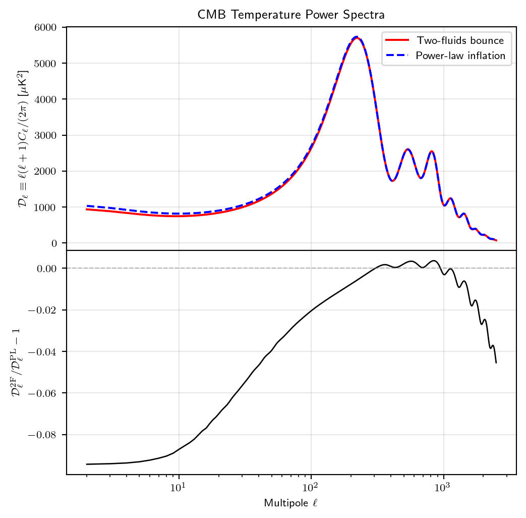
CMB Power Spectra Statistics:
  Two-fluids peak: 5699.38 μK² at ℓ = 221
  Power-law peak:  5732.85 μK² at ℓ = 220
  Ratio mean: -0.013678
  Ratio std:  0.015902
  Ratio range: [-0.094257, 0.003596]