import sys
import numpy as np
import math
import matplotlib.pyplot as plt
from IPython.display import HTML, Markdown, display

# CCL
import pyccl
import pandas as pd

# NumCosmo
from numcosmo_py import Nc, Ncm
from numcosmo_py.ccl.nc_ccl import create_nc_obj, CCLParams, dsigmaM_dlnM

from numcosmo_py.plotting.tools import set_rc_params_article, format_time
import numcosmo_py.cosmology as ncc
import numcosmo_py.ccl.comparison as nc_cmpBenchmarking NumCosmo vs. CCL
Abstract
This document compares the power spectrum implemented in NumCosmo and CCL.
Introduction
This notebook explores the power spectra and their derived quantities implemented in the Core Cosmology Library (CCL) and NumCosmo, two frameworks for computing cosmological observables. We aim to assess the consistency and accuracy of the matter power spectrum and related quantities, such as the linear growth factor and sigma_8, across these frameworks by comparing their outputs under identical physical parameters. To facilitate this analysis, we first establish a set of cosmological models with fixed and variable parameters, then define functions to compute and visualize the power spectra alongside their relative differences. The results are summarized in tables and plots below.
Initializing NumCosmo
To begin, we configure NumCosmo and redirect its output to this notebook using the following code:
Ncm.cfg_init()
Ncm.cfg_set_log_handler(lambda msg: sys.stdout.write(msg) and sys.stdout.flush())
set_rc_params_article(ncol=2, fontsize=12, use_tex=False)
Initial Parameter Definitions
We initialize the cosmological parameters and model-specific variables used for CCL and NumCosmo comparisons. Scalar parameters are fixed across all models, while arrays define variations in dark energy and neutrino properties for multiple scenarios. First, we instantiate a CCL cosmology object using the predefined global parameters. Next, using the numcosmo_py[^numcosmo_py] function create_nc_obj, we generate a NumCosmo cosmology object initialized with the same parameters as the CCL model. Fixed scalars apply universally, while arrays (\(\Omega_v\), \(w_0\), \(w_a\), \(m_\nu\)) represent different model configurations. Finally, in the setup_models function, one can enable high-precision computations in CCL, which increases accuracy at the cost of longer computation times. When this mode is activated, the overall agreement between CCL and NumCosmo improves significantly.
Code
from numcosmo_py.ccl.nc_ccl import create_nc_obj

PARAMETERS_SET = [
    r"$\Lambda$CDM, flat",
    r"$\Lambda$CDM, flat, $1\nu$",
    r"XCDM, flat",
    r"XCDM, spherical, $2\nu$",
    r"XCDM, hyperbolic",
]
COLORS = plt.rcParams["axes.prop_cycle"].by_key()["color"][:5]


def setup_models(
    Omega_c: float = 0.25,  # Cold dark matter density
    Omega_b: float = 0.05,  # Baryonic matter density
    h: float = 0.7,  # Dimensionless Hubble constant
    sigma8: float = 0.9,  # Matter density contrast std. dev. (8 Mpc/h)
    n_s: float = 0.96,  # Scalar spectral index
    Neff: float = 3.046,  # Effective number of massless neutrinos
    high_precision: bool = False,  # Use high precision computations in CCL
    dist_z_max: float = 15.0,  # Maximum redshift for distance computations
):
    """Setup cosmological models."""
    Omega_v_vals = np.array([0.7, 0.7, 0.7, 0.65, 0.75])  # Dark energy density
    w0_vals = np.array([-1.0, -1.0, -0.9, -0.9, -0.9])  # DE equation of state w0
    wa_vals = np.array([0.0, 0.0, 0.1, 0.1, 0.1])  # DE equation of state wa

    # Neutrino masses (eV) for each model: [m1, m2, m3]
    mnu = np.array(
        [
            [0.0, 0.0, 0.0],
            [0.04, 0.0, 0.0],
            [0.0, 0.0, 0.0],
            [0.03, 0.02, 0.0],
            [0.0, 0.0, 0.0],
        ]
    )
    Omega_k_vals = [
        float(1.0 - Omega_c - Omega_b - Omega_v) for Omega_v in Omega_v_vals
    ]

    parameters = [
        ["$\\Omega_c$", "Cold Dark Matter Density", Omega_c],
        ["$\\Omega_b$", "Baryonic Matter Density", Omega_b],
        ["$\\Omega_v$", "Dark Energy Density", Omega_v_vals],
        ["$\\Omega_k$", "Curvature Density", [f"{v:.3f}" for v in Omega_k_vals]],
        ["$h$", "Hubble Constant (dimensionless)", h],
        ["$n_s$", "Scalar Spectral Index", n_s],
        ["$N_\\mathrm{eff}$", "Effective Nº of Massless Neutrinos", Neff],
        ["$\\sigma_8$", "Matter Density Contrast Std. Dev. (8 Mpc/h)", sigma8],
        ["$w_0$", "DE Equation of State Parameter", w0_vals],
        ["$w_a$", "DE Equation of State Parameter", wa_vals],
        ["$m_\\nu$", "Neutrino Masses (eV)", [f"{m.tolist()}" for m in mnu]],
    ]
    models = []
    if high_precision:
        CCLParams.set_high_prec_params()

    for Omega_v, Omega_k, w0, wa, m in zip(
        Omega_v_vals, Omega_k_vals, w0_vals, wa_vals, mnu
    ):
        ccl_cosmo = pyccl.Cosmology(
            Omega_c=Omega_c,
            Omega_b=Omega_b,
            Neff=Neff,
            h=h,
            sigma8=sigma8,
            n_s=n_s,
            Omega_k=Omega_k,
            w0=w0,
            wa=wa,
            m_nu=m,
            transfer_function="eisenstein_hu",
        )
        cosmology = create_nc_obj(ccl_cosmo, dist_z_max=dist_z_max)
        models.append({"CCL": ccl_cosmo, "NC": cosmology})

    return parameters, models
# Preparing the models
parameters, models = setup_models(high_precision=False)
z = np.linspace(0.01, 15.0, 10000)Parameter Overview
The table below summarizes the parameters. There are five parameters sets.
Code
# Create DataFrame
df = pd.DataFrame(parameters, columns=["Symbol", "Description", "Value"])
display(Markdown(df.to_markdown(index=False, colalign=["left"] * len(df.columns))))| Symbol | Description | Value |
|---|---|---|
| \(\Omega_c\) | Cold Dark Matter Density | 0.25 |
| \(\Omega_b\) | Baryonic Matter Density | 0.05 |
| \(\Omega_v\) | Dark Energy Density | [0.7 0.7 0.7 0.65 0.75] |
| \(\Omega_k\) | Curvature Density | [‘0.000’, ‘0.000’, ‘0.000’, ‘0.050’, ‘-0.050’] |
| \(h\) | Hubble Constant (dimensionless) | 0.7 |
| \(n_s\) | Scalar Spectral Index | 0.96 |
| \(N_\mathrm{eff}\) | Effective Nº of Massless Neutrinos | 3.046 |
| \(\sigma_8\) | Matter Density Contrast Std. Dev. (8 Mpc/h) | 0.9 |
| \(w_0\) | DE Equation of State Parameter | [-1. -1. -0.9 -0.9 -0.9] |
| \(w_a\) | DE Equation of State Parameter | [0. 0. 0.1 0.1 0.1] |
| \(m_\nu\) | Neutrino Masses (eV) | [‘[0.0, 0.0, 0.0]’, ‘[0.04, 0.0, 0.0]’, ‘[0.0, 0.0, 0.0]’, ‘[0.03, 0.02, 0.0]’, ‘[0.0, 0.0, 0.0]’] |
Power Spectrum Comparison
The following code compares the power spectrum implemented in NumCosmo and CCL for a range of redshifts and wavenumbers.
ps_funcs = [
    nc_cmp.compare_power_spectrum_linear,
    nc_cmp.compare_power_spectrum_nonlinear,
]
z = np.array([0.0, 0.2, 0.5, 1.0, 2.0])
k = np.geomspace(5.0e-5, 1.0e3, 1000)

ps_comparisons: list[list[list[nc_cmp.CompareFunc1d]]] = [
    [
        [
            func(m["CCL"], m["NC"], k, z_i, model=name)
            for m, name in zip(models, PARAMETERS_SET)
        ]
        for func in ps_funcs
    ]
    for z_i in z
]
Code
for ps_comparison_z in ps_comparisons:
    for ps_comparison in ps_comparison_z:
        fig, axs = plt.subplots(2, sharex=True)
        fig.subplots_adjust(hspace=0)
        for p, c in zip(ps_comparison, COLORS):
            p.plot(axs=axs, color=c)
        axs[1].grid()
        plt.show()
plt.close()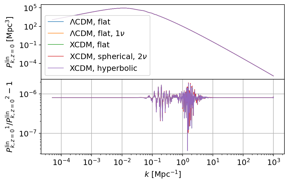
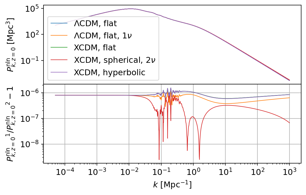
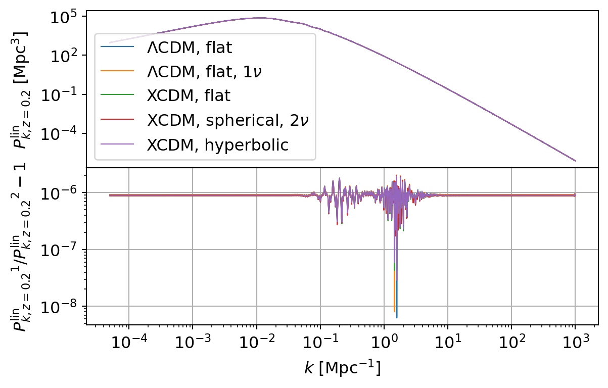
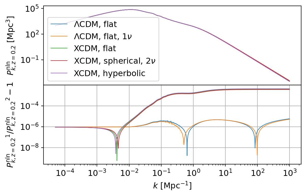
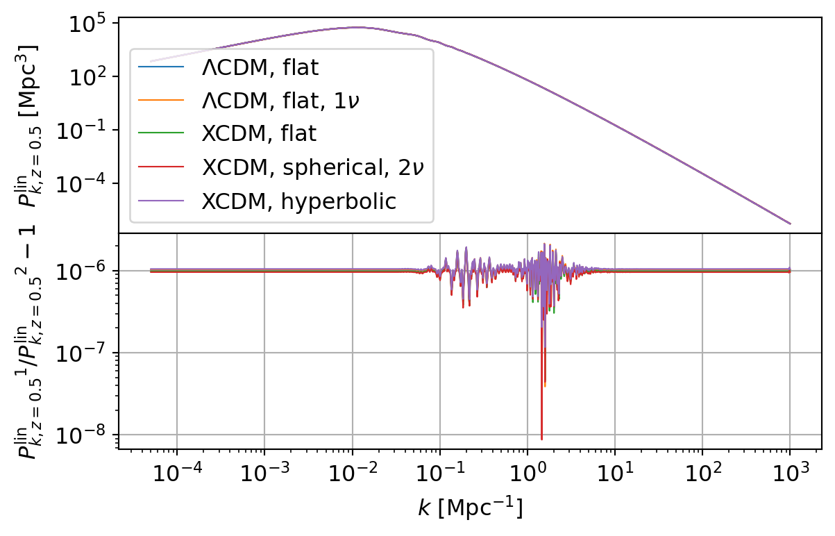
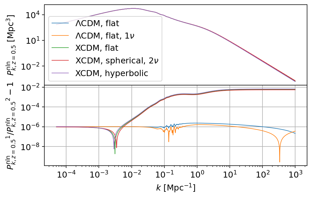
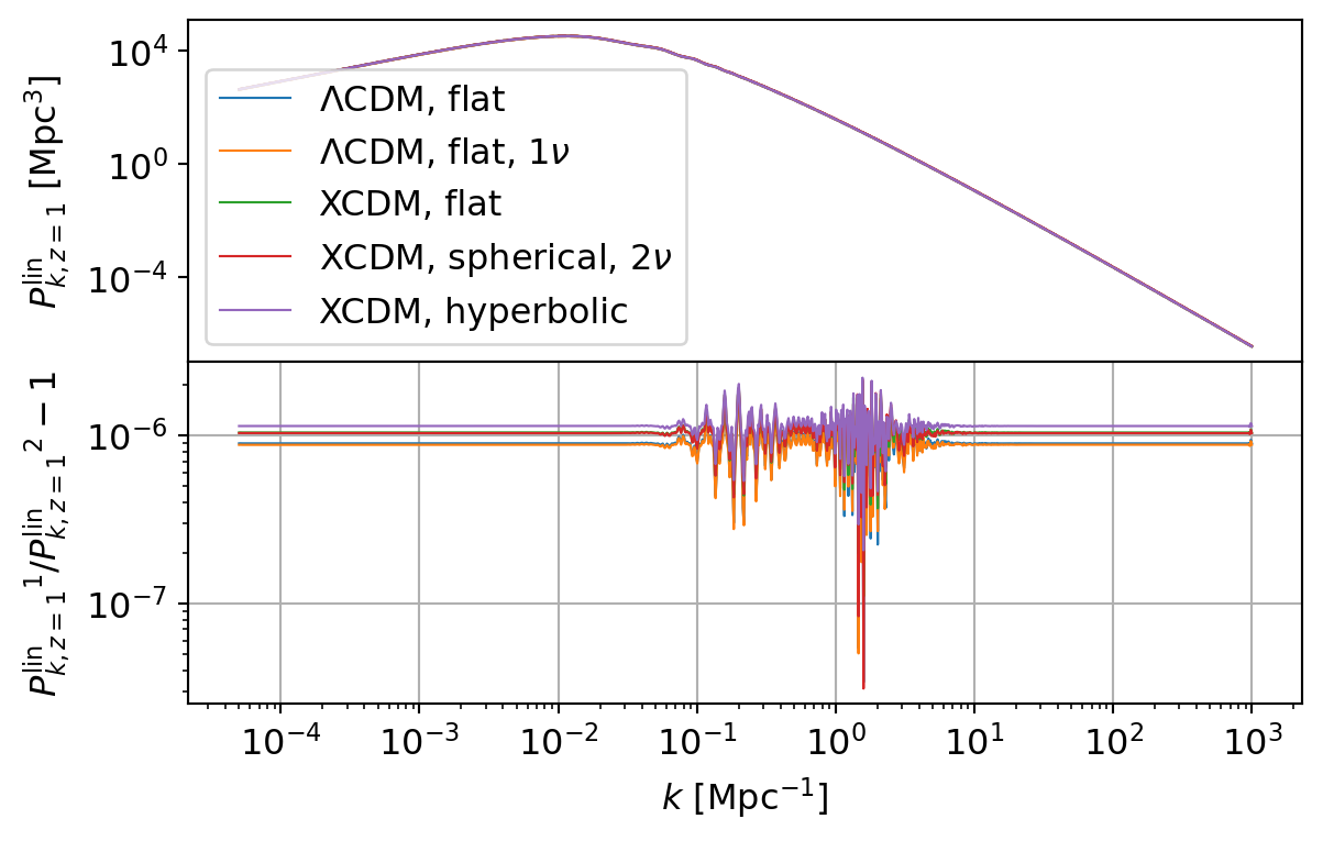
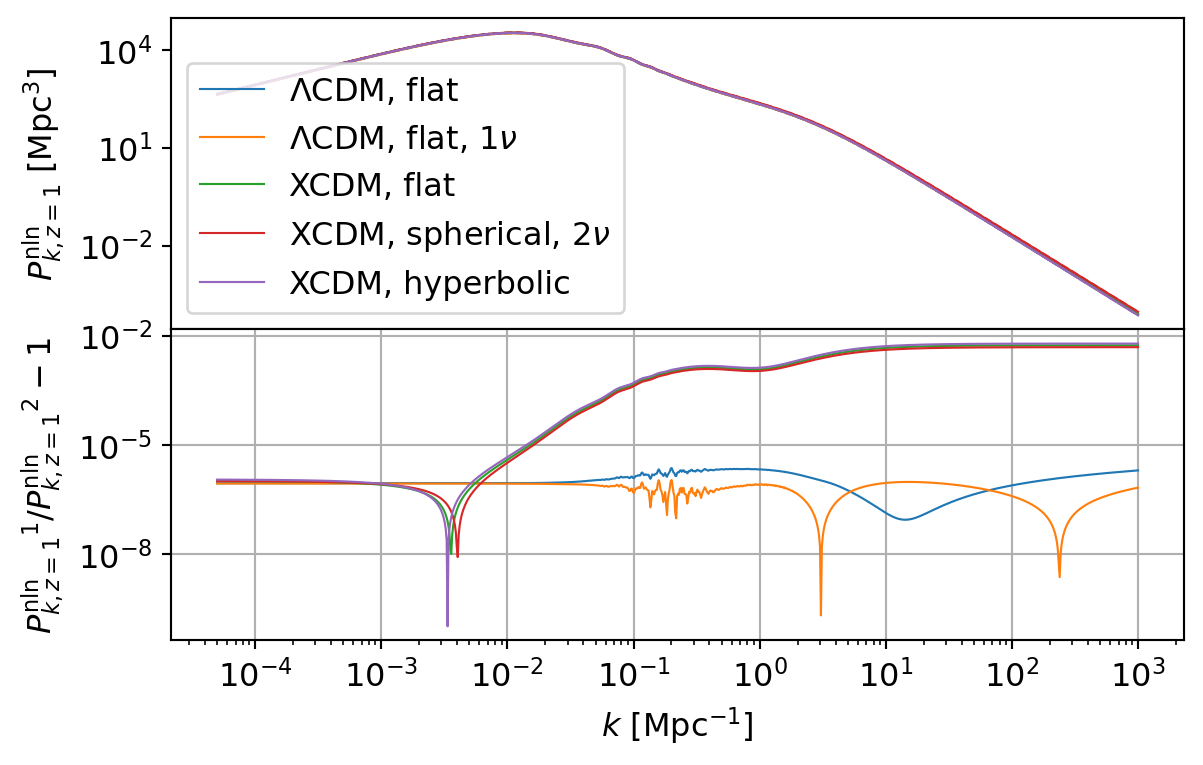
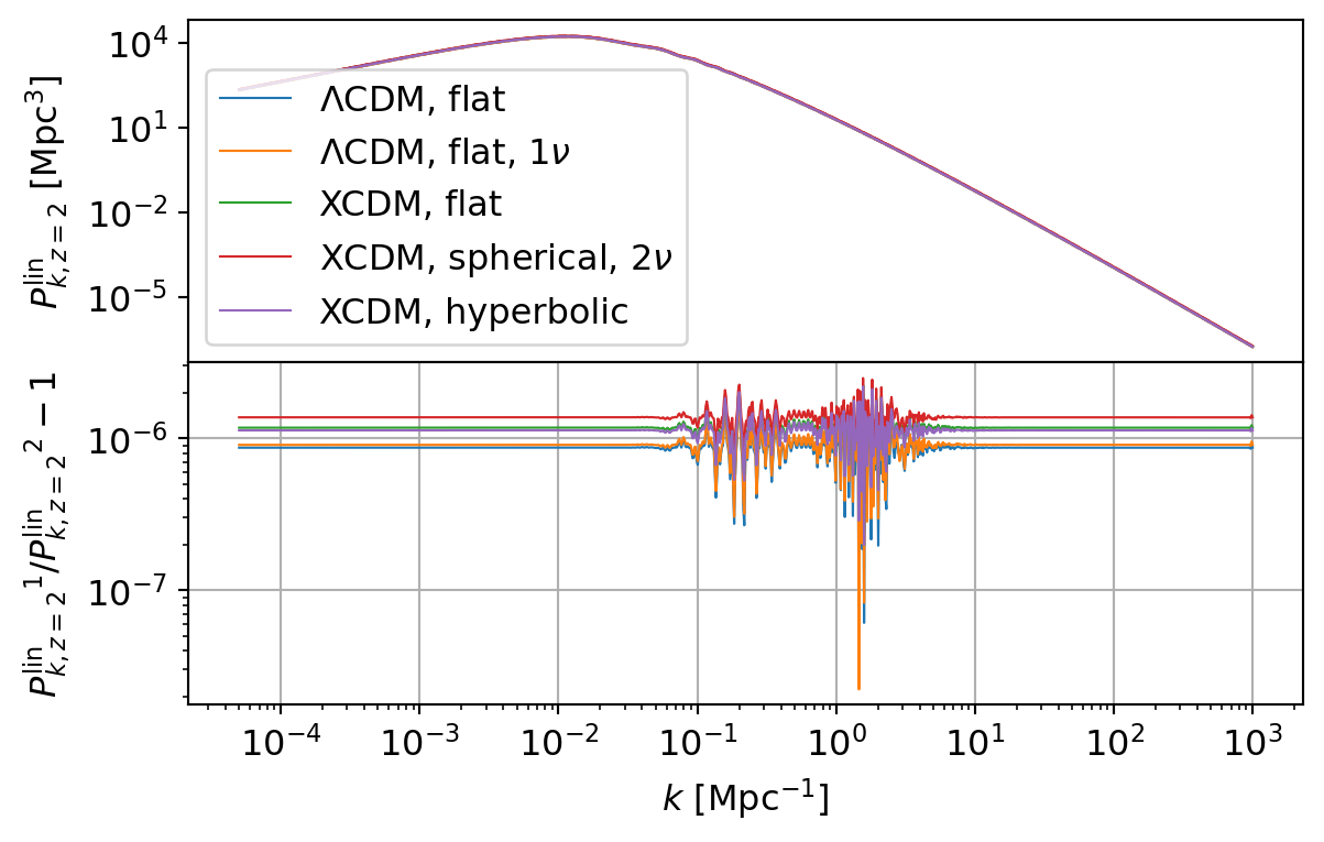
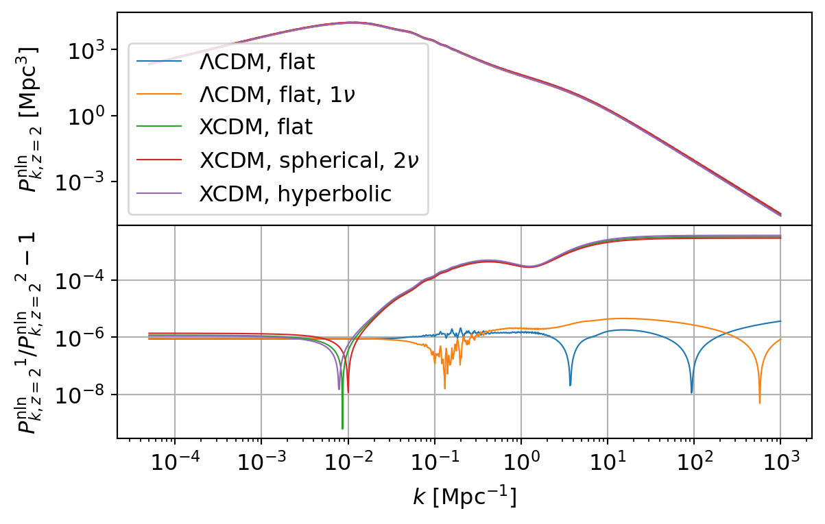
The following table summarizes the results for all sets.
Code
table = []

for ps_comparison_z in ps_comparisons:
    for ps_comparison in ps_comparison_z:
        for p in ps_comparison:
            table.append(p.summary_row(convert_g=False))

df = pd.DataFrame(table, columns=nc_cmp.CompareFunc1d.table_header())
display(Markdown(df.to_markdown(index=False, colalign=["left"] * len(df.columns))))| Model | Quantity | \(\Delta P_{\text{min}}/P\) | \(\Delta P_{\text{max}}/P\) | \(\overline{\Delta P / P}\) | \(\sigma_{\Delta P / P}\) |
|---|---|---|---|---|---|
| \(\Lambda\)CDM, flat | \({P_{k,z={0}}^\mathrm{lin}}\) [Mpc\({}^3\)] | \(3.58 \times 10^{-8}\) | \(1.87 \times 10^{-6}\) | \(8.06 \times 10^{-7}\) | \(1.32 \times 10^{-7}\) |
| \(\Lambda\)CDM, flat, \(1\nu\) | \({P_{k,z={0}}^\mathrm{lin}}\) [Mpc\({}^3\)] | \(1.05 \times 10^{-7}\) | \(1.92 \times 10^{-6}\) | \(8.09 \times 10^{-7}\) | \(1.34 \times 10^{-7}\) |
| XCDM, flat | \({P_{k,z={0}}^\mathrm{lin}}\) [Mpc\({}^3\)] | \(3.58 \times 10^{-8}\) | \(1.87 \times 10^{-6}\) | \(8.06 \times 10^{-7}\) | \(1.32 \times 10^{-7}\) |
| XCDM, spherical, \(2\nu\) | \({P_{k,z={0}}^\mathrm{lin}}\) [Mpc\({}^3\)] | \(1.03 \times 10^{-7}\) | \(1.93 \times 10^{-6}\) | \(8.11 \times 10^{-7}\) | \(1.34 \times 10^{-7}\) |
| XCDM, hyperbolic | \({P_{k,z={0}}^\mathrm{lin}}\) [Mpc\({}^3\)] | \(3.58 \times 10^{-8}\) | \(1.87 \times 10^{-6}\) | \(8.06 \times 10^{-7}\) | \(1.32 \times 10^{-7}\) |
| \(\Lambda\)CDM, flat | \({P_{k,z={0}}^\mathrm{nln}}\) [Mpc\({}^3\)] | \(5.98 \times 10^{-7}\) | \(1.56 \times 10^{-6}\) | \(8.12 \times 10^{-7}\) | \(1.45 \times 10^{-7}\) |
| \(\Lambda\)CDM, flat, \(1\nu\) | \({P_{k,z={0}}^\mathrm{nln}}\) [Mpc\({}^3\)] | \(2.89 \times 10^{-7}\) | \(1.18 \times 10^{-6}\) | \(6.69 \times 10^{-7}\) | \(1.65 \times 10^{-7}\) |
| XCDM, flat | \({P_{k,z={0}}^\mathrm{nln}}\) [Mpc\({}^3\)] | \(6.00 \times 10^{-7}\) | \(1.56 \times 10^{-6}\) | \(8.14 \times 10^{-7}\) | \(1.46 \times 10^{-7}\) |
| XCDM, spherical, \(2\nu\) | \({P_{k,z={0}}^\mathrm{nln}}\) [Mpc\({}^3\)] | \(2.43 \times 10^{-9}\) | \(9.66 \times 10^{-7}\) | \(4.61 \times 10^{-7}\) | \(2.94 \times 10^{-7}\) |
| XCDM, hyperbolic | \({P_{k,z={0}}^\mathrm{nln}}\) [Mpc\({}^3\)] | \(5.91 \times 10^{-7}\) | \(1.56 \times 10^{-6}\) | \(8.10 \times 10^{-7}\) | \(1.47 \times 10^{-7}\) |
| \(\Lambda\)CDM, flat | \({P_{k,z={0.2}}^\mathrm{lin}}\) [Mpc\({}^3\)] | \(6.23 \times 10^{-9}\) | \(1.99 \times 10^{-6}\) | \(9.24 \times 10^{-7}\) | \(1.34 \times 10^{-7}\) |
| \(\Lambda\)CDM, flat, \(1\nu\) | \({P_{k,z={0.2}}^\mathrm{lin}}\) [Mpc\({}^3\)] | \(8.07 \times 10^{-9}\) | \(2.03 \times 10^{-6}\) | \(9.22 \times 10^{-7}\) | \(1.36 \times 10^{-7}\) |
| XCDM, flat | \({P_{k,z={0.2}}^\mathrm{lin}}\) [Mpc\({}^3\)] | \(4.28 \times 10^{-8}\) | \(1.95 \times 10^{-6}\) | \(8.85 \times 10^{-7}\) | \(1.33 \times 10^{-7}\) |
| XCDM, spherical, \(2\nu\) | \({P_{k,z={0.2}}^\mathrm{lin}}\) [Mpc\({}^3\)] | \(7.00 \times 10^{-8}\) | \(1.99 \times 10^{-6}\) | \(8.79 \times 10^{-7}\) | \(1.36 \times 10^{-7}\) |
| XCDM, hyperbolic | \({P_{k,z={0.2}}^\mathrm{lin}}\) [Mpc\({}^3\)] | \(2.87 \times 10^{-8}\) | \(1.97 \times 10^{-6}\) | \(9.01 \times 10^{-7}\) | \(1.34 \times 10^{-7}\) |
| \(\Lambda\)CDM, flat | \({P_{k,z={0.2}}^\mathrm{nln}}\) [Mpc\({}^3\)] | \(1.67 \times 10^{-9}\) | \(5.70 \times 10^{-6}\) | \(2.00 \times 10^{-6}\) | \(1.39 \times 10^{-6}\) |
| \(\Lambda\)CDM, flat, \(1\nu\) | \({P_{k,z={0.2}}^\mathrm{nln}}\) [Mpc\({}^3\)] | \(1.88 \times 10^{-9}\) | \(5.03 \times 10^{-6}\) | \(1.89 \times 10^{-6}\) | \(1.31 \times 10^{-6}\) |
| XCDM, flat | \({P_{k,z={0.2}}^\mathrm{nln}}\) [Mpc\({}^3\)] | \(5.44 \times 10^{-10}\) | \(3.95 \times 10^{-3}\) | \(1.64 \times 10^{-3}\) | \(1.68 \times 10^{-3}\) |
| XCDM, spherical, \(2\nu\) | \({P_{k,z={0.2}}^\mathrm{nln}}\) [Mpc\({}^3\)] | \(8.35 \times 10^{-9}\) | \(3.61 \times 10^{-3}\) | \(1.49 \times 10^{-3}\) | \(1.53 \times 10^{-3}\) |
| XCDM, hyperbolic | \({P_{k,z={0.2}}^\mathrm{nln}}\) [Mpc\({}^3\)] | \(2.55 \times 10^{-9}\) | \(4.30 \times 10^{-3}\) | \(1.79 \times 10^{-3}\) | \(1.83 \times 10^{-3}\) |
| \(\Lambda\)CDM, flat | \({P_{k,z={0.5}}^\mathrm{lin}}\) [Mpc\({}^3\)] | \(9.12 \times 10^{-8}\) | \(2.09 \times 10^{-6}\) | \(1.02 \times 10^{-6}\) | \(1.34 \times 10^{-7}\) |
| \(\Lambda\)CDM, flat, \(1\nu\) | \({P_{k,z={0.5}}^\mathrm{lin}}\) [Mpc\({}^3\)] | \(3.86 \times 10^{-8}\) | \(2.14 \times 10^{-6}\) | \(1.03 \times 10^{-6}\) | \(1.38 \times 10^{-7}\) |
| XCDM, flat | \({P_{k,z={0.5}}^\mathrm{lin}}\) [Mpc\({}^3\)] | \(4.62 \times 10^{-8}\) | \(2.04 \times 10^{-6}\) | \(9.76 \times 10^{-7}\) | \(1.34 \times 10^{-7}\) |
| XCDM, spherical, \(2\nu\) | \({P_{k,z={0.5}}^\mathrm{lin}}\) [Mpc\({}^3\)] | \(8.72 \times 10^{-9}\) | \(2.07 \times 10^{-6}\) | \(9.57 \times 10^{-7}\) | \(1.38 \times 10^{-7}\) |
| XCDM, hyperbolic | \({P_{k,z={0.5}}^\mathrm{lin}}\) [Mpc\({}^3\)] | \(1.17 \times 10^{-7}\) | \(2.11 \times 10^{-6}\) | \(1.05 \times 10^{-6}\) | \(1.34 \times 10^{-7}\) |
| \(\Lambda\)CDM, flat | \({P_{k,z={0.5}}^\mathrm{nln}}\) [Mpc\({}^3\)] | \(2.09 \times 10^{-7}\) | \(2.35 \times 10^{-6}\) | \(1.26 \times 10^{-6}\) | \(5.34 \times 10^{-7}\) |
| \(\Lambda\)CDM, flat, \(1\nu\) | \({P_{k,z={0.5}}^\mathrm{nln}}\) [Mpc\({}^3\)] | \(2.66 \times 10^{-10}\) | \(1.64 \times 10^{-6}\) | \(8.98 \times 10^{-7}\) | \(4.05 \times 10^{-7}\) |
| XCDM, flat | \({P_{k,z={0.5}}^\mathrm{nln}}\) [Mpc\({}^3\)] | \(1.81 \times 10^{-9}\) | \(5.97 \times 10^{-3}\) | \(2.37 \times 10^{-3}\) | \(2.51 \times 10^{-3}\) |
| XCDM, spherical, \(2\nu\) | \({P_{k,z={0.5}}^\mathrm{nln}}\) [Mpc\({}^3\)] | \(7.40 \times 10^{-9}\) | \(5.37 \times 10^{-3}\) | \(2.13 \times 10^{-3}\) | \(2.26 \times 10^{-3}\) |
| XCDM, hyperbolic | \({P_{k,z={0.5}}^\mathrm{nln}}\) [Mpc\({}^3\)] | \(5.62 \times 10^{-9}\) | \(6.60 \times 10^{-3}\) | \(2.62 \times 10^{-3}\) | \(2.78 \times 10^{-3}\) |
| \(\Lambda\)CDM, flat | \({P_{k,z={1}}^\mathrm{lin}}\) [Mpc\({}^3\)] | \(3.39 \times 10^{-8}\) | \(1.96 \times 10^{-6}\) | \(8.96 \times 10^{-7}\) | \(1.34 \times 10^{-7}\) |
| \(\Lambda\)CDM, flat, \(1\nu\) | \({P_{k,z={1}}^\mathrm{lin}}\) [Mpc\({}^3\)] | \(5.03 \times 10^{-8}\) | \(1.99 \times 10^{-6}\) | \(8.80 \times 10^{-7}\) | \(1.35 \times 10^{-7}\) |
| XCDM, flat | \({P_{k,z={1}}^\mathrm{lin}}\) [Mpc\({}^3\)] | \(1.10 \times 10^{-7}\) | \(2.11 \times 10^{-6}\) | \(1.04 \times 10^{-6}\) | \(1.34 \times 10^{-7}\) |
| XCDM, spherical, \(2\nu\) | \({P_{k,z={1}}^\mathrm{lin}}\) [Mpc\({}^3\)] | \(3.11 \times 10^{-8}\) | \(2.15 \times 10^{-6}\) | \(1.03 \times 10^{-6}\) | \(1.38 \times 10^{-7}\) |
| XCDM, hyperbolic | \({P_{k,z={1}}^\mathrm{lin}}\) [Mpc\({}^3\)] | \(2.07 \times 10^{-7}\) | \(2.20 \times 10^{-6}\) | \(1.14 \times 10^{-6}\) | \(1.34 \times 10^{-7}\) |
| \(\Lambda\)CDM, flat | \({P_{k,z={1}}^\mathrm{nln}}\) [Mpc\({}^3\)] | \(8.85 \times 10^{-8}\) | \(2.35 \times 10^{-6}\) | \(1.07 \times 10^{-6}\) | \(5.45 \times 10^{-7}\) |
| \(\Lambda\)CDM, flat, \(1\nu\) | \({P_{k,z={1}}^\mathrm{nln}}\) [Mpc\({}^3\)] | \(2.07 \times 10^{-10}\) | \(1.10 \times 10^{-6}\) | \(6.88 \times 10^{-7}\) | \(2.56 \times 10^{-7}\) |
| XCDM, flat | \({P_{k,z={1}}^\mathrm{nln}}\) [Mpc\({}^3\)] | \(1.01 \times 10^{-8}\) | \(5.56 \times 10^{-3}\) | \(2.04 \times 10^{-3}\) | \(2.32 \times 10^{-3}\) |
| XCDM, spherical, \(2\nu\) | \({P_{k,z={1}}^\mathrm{nln}}\) [Mpc\({}^3\)] | \(8.31 \times 10^{-9}\) | \(4.95 \times 10^{-3}\) | \(1.82 \times 10^{-3}\) | \(2.06 \times 10^{-3}\) |
| XCDM, hyperbolic | \({P_{k,z={1}}^\mathrm{nln}}\) [Mpc\({}^3\)] | \(1.03 \times 10^{-10}\) | \(6.21 \times 10^{-3}\) | \(2.28 \times 10^{-3}\) | \(2.59 \times 10^{-3}\) |
| \(\Lambda\)CDM, flat | \({P_{k,z={2}}^\mathrm{lin}}\) [Mpc\({}^3\)] | \(2.68 \times 10^{-8}\) | \(1.94 \times 10^{-6}\) | \(8.69 \times 10^{-7}\) | \(1.33 \times 10^{-7}\) |
| \(\Lambda\)CDM, flat, \(1\nu\) | \({P_{k,z={2}}^\mathrm{lin}}\) [Mpc\({}^3\)] | \(2.22 \times 10^{-8}\) | \(2.02 \times 10^{-6}\) | \(9.08 \times 10^{-7}\) | \(1.36 \times 10^{-7}\) |
| XCDM, flat | \({P_{k,z={2}}^\mathrm{lin}}\) [Mpc\({}^3\)] | \(2.46 \times 10^{-7}\) | \(2.24 \times 10^{-6}\) | \(1.18 \times 10^{-6}\) | \(1.34 \times 10^{-7}\) |
| XCDM, spherical, \(2\nu\) | \({P_{k,z={2}}^\mathrm{lin}}\) [Mpc\({}^3\)] | \(3.75 \times 10^{-7}\) | \(2.49 \times 10^{-6}\) | \(1.38 \times 10^{-6}\) | \(1.38 \times 10^{-7}\) |
| XCDM, hyperbolic | \({P_{k,z={2}}^\mathrm{lin}}\) [Mpc\({}^3\)] | \(1.99 \times 10^{-7}\) | \(2.20 \times 10^{-6}\) | \(1.13 \times 10^{-6}\) | \(1.34 \times 10^{-7}\) |
| \(\Lambda\)CDM, flat | \({P_{k,z={2}}^\mathrm{nln}}\) [Mpc\({}^3\)] | \(1.13 \times 10^{-8}\) | \(3.64 \times 10^{-6}\) | \(1.15 \times 10^{-6}\) | \(5.79 \times 10^{-7}\) |
| \(\Lambda\)CDM, flat, \(1\nu\) | \({P_{k,z={2}}^\mathrm{nln}}\) [Mpc\({}^3\)] | \(4.93 \times 10^{-9}\) | \(4.50 \times 10^{-6}\) | \(1.61 \times 10^{-6}\) | \(1.23 \times 10^{-6}\) |
| XCDM, flat | \({P_{k,z={2}}^\mathrm{nln}}\) [Mpc\({}^3\)] | \(6.21 \times 10^{-10}\) | \(3.23 \times 10^{-3}\) | \(1.03 \times 10^{-3}\) | \(1.32 \times 10^{-3}\) |
| XCDM, spherical, \(2\nu\) | \({P_{k,z={2}}^\mathrm{nln}}\) [Mpc\({}^3\)] | \(1.17 \times 10^{-8}\) | \(2.88 \times 10^{-3}\) | \(9.25 \times 10^{-4}\) | \(1.18 \times 10^{-3}\) |
| XCDM, hyperbolic | \({P_{k,z={2}}^\mathrm{nln}}\) [Mpc\({}^3\)] | \(1.50 \times 10^{-8}\) | \(3.60 \times 10^{-3}\) | \(1.15 \times 10^{-3}\) | \(1.48 \times 10^{-3}\) |
Matter Density Variance
The following code compares the variance of the matter density averaged over a sphere of radius \(r\) for a range of redshifts.
z = np.array([0.0, 0.2, 0.5, 1.0, 2.0, 6.0])
r = np.geomspace(1.0e-1, 1.0e1, 1000)

compare_variances: list[nc_cmp.CompareFunc1d] = [
    [
        nc_cmp.compare_sigma_r(m["CCL"], m["NC"], r, z_i, model=name)
        for m, name in zip(models, PARAMETERS_SET)
    ]
    for z_i in z
]
Code
for compare_variance_z in compare_variances:
    fig, axs = plt.subplots(2, sharex=True)
    fig.subplots_adjust(hspace=0)
    for p, c in zip(compare_variance_z, COLORS):
        p.plot(axs=axs, color=c)
    axs[1].grid()
    plt.show()
plt.close()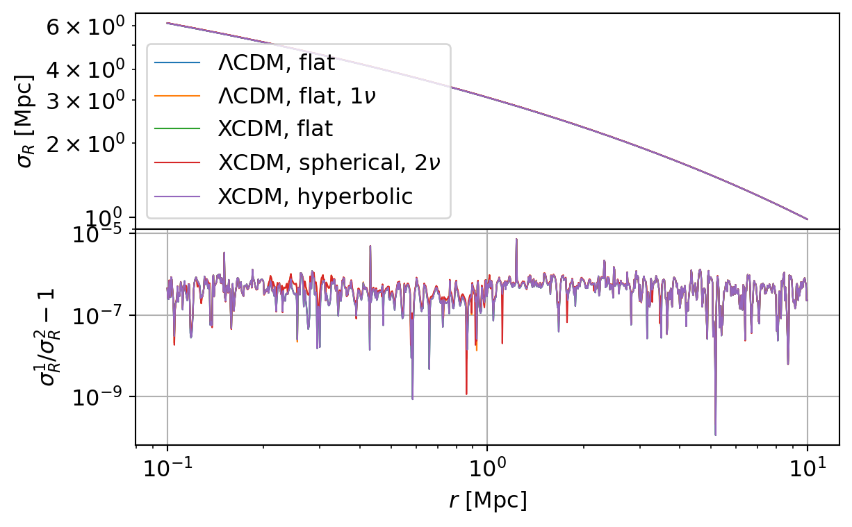
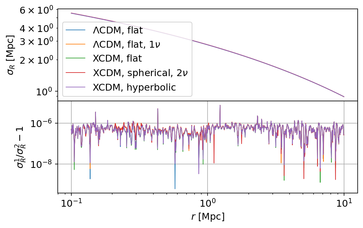
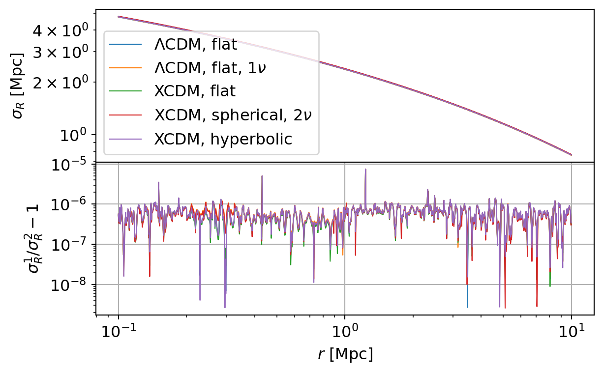
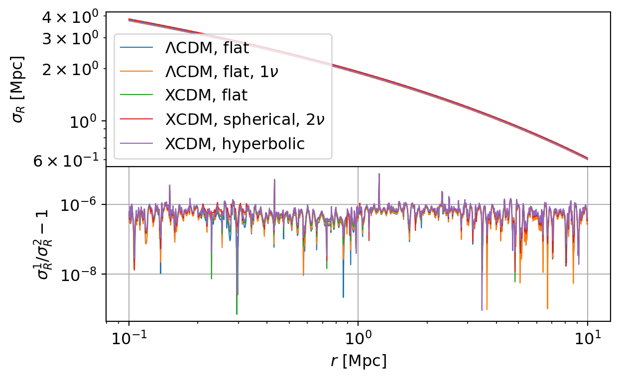
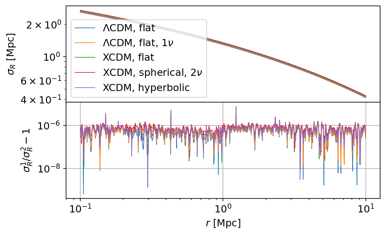
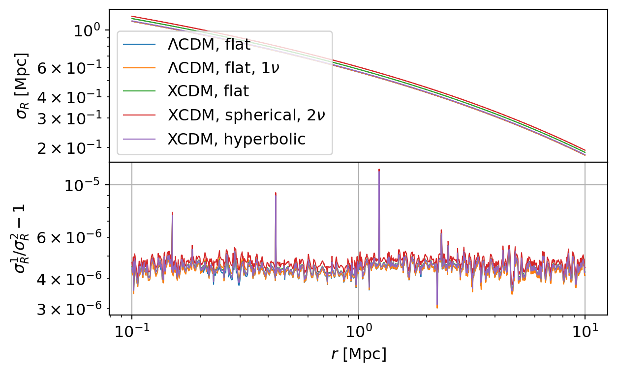
The following table summarizes the results for all parameter sets.
Code
table = []

for compare_variance_z in compare_variances:
    for d in compare_variance_z:
        table.append(d.summary_row(convert_g=False))

df = pd.DataFrame(table, columns=nc_cmp.CompareFunc1d.table_header())
display(Markdown(df.to_markdown(index=False, colalign=["left"] * len(df.columns))))| Model | Quantity | \(\Delta P_{\text{min}}/P\) | \(\Delta P_{\text{max}}/P\) | \(\overline{\Delta P / P}\) | \(\sigma_{\Delta P / P}\) |
|---|---|---|---|---|---|
| \(\Lambda\)CDM, flat | \(\sigma_R\) [Mpc] | \(1.14 \times 10^{-10}\) | \(7.35 \times 10^{-6}\) | \(4.72 \times 10^{-7}\) | \(3.75 \times 10^{-7}\) |
| \(\Lambda\)CDM, flat, \(1\nu\) | \(\sigma_R\) [Mpc] | \(2.60 \times 10^{-10}\) | \(7.38 \times 10^{-6}\) | \(5.02 \times 10^{-7}\) | \(3.75 \times 10^{-7}\) |
| XCDM, flat | \(\sigma_R\) [Mpc] | \(1.14 \times 10^{-10}\) | \(7.35 \times 10^{-6}\) | \(4.72 \times 10^{-7}\) | \(3.75 \times 10^{-7}\) |
| XCDM, spherical, \(2\nu\) | \(\sigma_R\) [Mpc] | \(2.08 \times 10^{-10}\) | \(7.39 \times 10^{-6}\) | \(5.05 \times 10^{-7}\) | \(3.75 \times 10^{-7}\) |
| XCDM, hyperbolic | \(\sigma_R\) [Mpc] | \(1.14 \times 10^{-10}\) | \(7.35 \times 10^{-6}\) | \(4.72 \times 10^{-7}\) | \(3.75 \times 10^{-7}\) |
| \(\Lambda\)CDM, flat | \(\sigma_R\) [Mpc] | \(6.23 \times 10^{-10}\) | \(7.41 \times 10^{-6}\) | \(5.22 \times 10^{-7}\) | \(3.78 \times 10^{-7}\) |
| \(\Lambda\)CDM, flat, \(1\nu\) | \(\sigma_R\) [Mpc] | \(5.97 \times 10^{-9}\) | \(7.43 \times 10^{-6}\) | \(5.50 \times 10^{-7}\) | \(3.78 \times 10^{-7}\) |
| XCDM, flat | \(\sigma_R\) [Mpc] | \(1.28 \times 10^{-9}\) | \(7.39 \times 10^{-6}\) | \(5.05 \times 10^{-7}\) | \(3.77 \times 10^{-7}\) |
| XCDM, spherical, \(2\nu\) | \(\sigma_R\) [Mpc] | \(1.75 \times 10^{-9}\) | \(7.42 \times 10^{-6}\) | \(5.34 \times 10^{-7}\) | \(3.77 \times 10^{-7}\) |
| XCDM, hyperbolic | \(\sigma_R\) [Mpc] | \(3.35 \times 10^{-9}\) | \(7.40 \times 10^{-6}\) | \(5.12 \times 10^{-7}\) | \(3.78 \times 10^{-7}\) |
| \(\Lambda\)CDM, flat | \(\sigma_R\) [Mpc] | \(2.68 \times 10^{-9}\) | \(7.46 \times 10^{-6}\) | \(5.73 \times 10^{-7}\) | \(3.81 \times 10^{-7}\) |
| \(\Lambda\)CDM, flat, \(1\nu\) | \(\sigma_R\) [Mpc] | \(1.29 \times 10^{-8}\) | \(7.49 \times 10^{-6}\) | \(6.07 \times 10^{-7}\) | \(3.80 \times 10^{-7}\) |
| XCDM, flat | \(\sigma_R\) [Mpc] | \(8.88 \times 10^{-9}\) | \(7.44 \times 10^{-6}\) | \(5.51 \times 10^{-7}\) | \(3.80 \times 10^{-7}\) |
| XCDM, spherical, \(2\nu\) | \(\sigma_R\) [Mpc] | \(2.58 \times 10^{-9}\) | \(7.46 \times 10^{-6}\) | \(5.74 \times 10^{-7}\) | \(3.79 \times 10^{-7}\) |
| XCDM, hyperbolic | \(\sigma_R\) [Mpc] | \(2.62 \times 10^{-9}\) | \(7.47 \times 10^{-6}\) | \(5.85 \times 10^{-7}\) | \(3.82 \times 10^{-7}\) |
| \(\Lambda\)CDM, flat | \(\sigma_R\) [Mpc] | \(2.16 \times 10^{-9}\) | \(7.40 \times 10^{-6}\) | \(5.14 \times 10^{-7}\) | \(3.78 \times 10^{-7}\) |
| \(\Lambda\)CDM, flat, \(1\nu\) | \(\sigma_R\) [Mpc] | \(9.73 \times 10^{-10}\) | \(7.42 \times 10^{-6}\) | \(5.35 \times 10^{-7}\) | \(3.77 \times 10^{-7}\) |
| XCDM, flat | \(\sigma_R\) [Mpc] | \(7.14 \times 10^{-10}\) | \(7.47 \times 10^{-6}\) | \(5.82 \times 10^{-7}\) | \(3.81 \times 10^{-7}\) |
| XCDM, spherical, \(2\nu\) | \(\sigma_R\) [Mpc] | \(1.18 \times 10^{-8}\) | \(7.50 \times 10^{-6}\) | \(6.10 \times 10^{-7}\) | \(3.81 \times 10^{-7}\) |
| XCDM, hyperbolic | \(\sigma_R\) [Mpc] | \(9.19 \times 10^{-10}\) | \(7.52 \times 10^{-6}\) | \(6.29 \times 10^{-7}\) | \(3.83 \times 10^{-7}\) |
| \(\Lambda\)CDM, flat | \(\sigma_R\) [Mpc] | \(6.44 \times 10^{-10}\) | \(7.38 \times 10^{-6}\) | \(5.01 \times 10^{-7}\) | \(3.77 \times 10^{-7}\) |
| \(\Lambda\)CDM, flat, \(1\nu\) | \(\sigma_R\) [Mpc] | \(7.86 \times 10^{-9}\) | \(7.43 \times 10^{-6}\) | \(5.49 \times 10^{-7}\) | \(3.78 \times 10^{-7}\) |
| XCDM, flat | \(\sigma_R\) [Mpc] | \(1.21 \times 10^{-8}\) | \(7.54 \times 10^{-6}\) | \(6.48 \times 10^{-7}\) | \(3.84 \times 10^{-7}\) |
| XCDM, spherical, \(2\nu\) | \(\sigma_R\) [Mpc] | \(8.04 \times 10^{-9}\) | \(7.67 \times 10^{-6}\) | \(7.78 \times 10^{-7}\) | \(3.86 \times 10^{-7}\) |
| XCDM, hyperbolic | \(\sigma_R\) [Mpc] | \(1.31 \times 10^{-9}\) | \(7.51 \times 10^{-6}\) | \(6.25 \times 10^{-7}\) | \(3.83 \times 10^{-7}\) |
| \(\Lambda\)CDM, flat | \(\sigma_R\) [Mpc] | \(3.01 \times 10^{-6}\) | \(1.13 \times 10^{-5}\) | \(4.37 \times 10^{-6}\) | \(3.92 \times 10^{-7}\) |
| \(\Lambda\)CDM, flat, \(1\nu\) | \(\sigma_R\) [Mpc] | \(3.01 \times 10^{-6}\) | \(1.13 \times 10^{-5}\) | \(4.39 \times 10^{-6}\) | \(3.92 \times 10^{-7}\) |
| XCDM, flat | \(\sigma_R\) [Mpc] | \(3.14 \times 10^{-6}\) | \(1.14 \times 10^{-5}\) | \(4.50 \times 10^{-6}\) | \(3.92 \times 10^{-7}\) |
| XCDM, spherical, \(2\nu\) | \(\sigma_R\) [Mpc] | \(3.35 \times 10^{-6}\) | \(1.16 \times 10^{-5}\) | \(4.73 \times 10^{-6}\) | \(3.91 \times 10^{-7}\) |
| XCDM, hyperbolic | \(\sigma_R\) [Mpc] | \(3.11 \times 10^{-6}\) | \(1.14 \times 10^{-5}\) | \(4.47 \times 10^{-6}\) | \(3.92 \times 10^{-7}\) |