import numpy as np
import matplotlib.pyplot as plt
from scipy.stats import norm

from numcosmo_py import Ncm

# Initialize the library
Ncm.cfg_init()Empirical Probability Density Function (EPDF) Example
Abstract
This document demonstrates how to use the Ncm.StatsDist1dEPDF object from the numcosmo library to compute the probability density function (PDF) and cumulative distribution function (CDF) of a distribution of points. The example uses a Gaussian mixture distribution and compares the results with the true distribution.
Introduction
This example demonstrates how to use the Ncm.StatsDist1dEPDF object from the numcosmo library to compute the probability density function (PDF) and cumulative distribution function (CDF) of a distribution of points. We generate a sample from a Gaussian mixture distribution, reconstruct the PDF and CDF using the numcosmo library, and compare the results with the true distribution. This guide assumes familiarity with probability distributions and basic Python programming.
Prerequisites
Before running this example, make sure the numcosmo_py1 package is installed in your environment. If it is not already installed, follow the installation instructions in the NumCosmo documentation. In addition, we are using numpy, matplotlib, and scipy.stats for data manipulation and plotting. If you are using the conda installation, these packages are already installed.
1 NumCosmo is a C library for cosmology and astrophysics that uses GObject-Introspection to provide bindings for various programming languages. To improve the user interface, we provide a Python package, numcosmo_py. This package imports all NumCosmo bindings and includes additional helper functions to simplify library usage.
Import and Initialize
First, import the required modules and initialize the NumCosmo library. The Ncm module provides the core functionality of the NumCosmo library. The call to Ncm.cfg_init() initializes the library objects.
Generating the Sample
We generate a sample from a Gaussian mixture distribution with two peaks. The sample is then filtered to include only points within a specified range.
# Set the random seed for reproducibility
np.random.seed(0)

# Define the parameters of the Gaussian mixture distribution
cut_l = -0.6  # Lower cutoff
cut_u = 0.6  # Upper cutoff
peak1 = -0.1  # Mean of the first Gaussian
sigma1 = 0.05  # Standard deviation of the first Gaussian
peak2 = 0.1  # Mean of the second Gaussian
sigma2 = 0.05  # Standard deviation of the second Gaussian


# Define the true cumulative distribution function (CDF)
def true_cdf(x):
    """Compute the true cumulative distribution function."""
    return 0.5 * (norm.cdf(x, peak1, sigma1) + norm.cdf(x, peak2, sigma2))


# Compute the normalization factor for the truncated distribution
cdf_cut_l = true_cdf(cut_l)
cdf_cut_u = 1.0 - true_cdf(cut_u)
cdf_cut = cdf_cut_l + cdf_cut_u
rb_norm = 1.0 - cdf_cut


# Define the true probability density function (PDF)
def true_p(x):
    """Compute the true probability density function."""
    return 0.5 * (norm.pdf(x, peak1, sigma1) + norm.pdf(x, peak2, sigma2)) / rb_norm


# Generate the sample
n = 4000
s = np.concatenate(
    (np.random.normal(peak1, sigma1, n), np.random.normal(peak2, sigma2, n)), axis=0
)

# Filter the sample to include only points within the specified range
sa = [si for si in s if si >= cut_l and si <= cut_u]
s = np.array(sa)
n = len(s)

print(f"# Number of points = {n}")
# Number of points = 8000Reconstructing the PDF and CDF
We use the Ncm.StatsDist1dEPDF object to reconstruct the PDF and CDF from the sample. Two methods are used for bandwidth selection: automatic bandwidth selection (AUTO) and the rule-of-thumb (ROT).
# Create the EPDF objects
epdf = Ncm.StatsDist1dEPDF.new_full(2000, Ncm.StatsDist1dEPDFBw.AUTO, 0.01, 0.001)
epdf_rot = Ncm.StatsDist1dEPDF.new_full(2000, Ncm.StatsDist1dEPDFBw.ROT, 0.01, 0.001)

# Add the points to the EPDF objects
for i in range(n):
    epdf.add_obs(s[i])
    epdf_rot.add_obs(s[i])

# Prepare the EPDF objects
epdf.prepare()
epdf_rot.prepare()
Plotting the Results
We plot the reconstructed PDF, CDF, and inverse CDF, and compare them with the true distribution.
Probability Density Function (PDF)
Code
# Compute the PDF for plotting
x_a = np.linspace(epdf.get_xi(), epdf.get_xf(), 1000)
p_a = [epdf.eval_p(x) for x in x_a]
p_rot_a = [epdf_rot.eval_p(x) for x in x_a]
pdf_true = true_p(x_a)

# Plot the PDF
plt.figure(figsize=(10, 6))
plt.title("PDF")
plt.plot(x_a, p_a, label="auto-bw")
plt.plot(x_a, p_rot_a, label="RoT-bw")
plt.plot(x_a, pdf_true, label="true dist")
plt.legend(loc="best")
plt.show()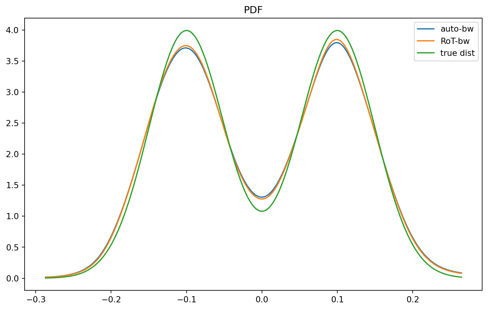
Relative Difference in PDF
Code
# Compute the relative difference
rel_diff_auto = np.abs((p_a - pdf_true) / pdf_true)
rel_diff_rot = np.abs((p_rot_a - pdf_true) / pdf_true)

# Plot the relative difference
plt.figure(figsize=(10, 6))
plt.title("PDF relative difference with respect to the true distribution")
plt.plot(x_a, rel_diff_auto, label="auto-bw")
plt.plot(x_a, rel_diff_rot, label="RoT-bw")
plt.ylim((1.0e-6, 1.0e1))
plt.grid()
plt.legend(loc="best")
plt.yscale("log")
plt.show()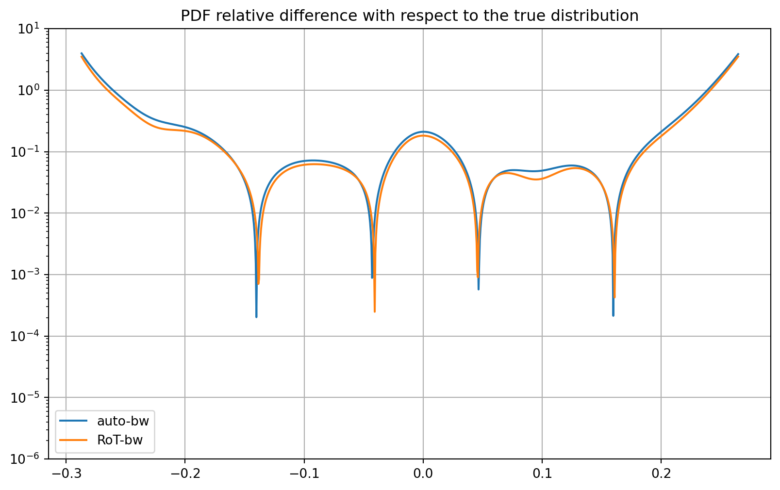
Cumulative Distribution Function (CDF)
Code
# Compute the CDF for plotting
pdf_a = [epdf.eval_pdf(x) for x in x_a]
pdf_rot_a = [epdf_rot.eval_pdf(x) for x in x_a]
cdf_true = (true_cdf(x_a) - cdf_cut_l) / rb_norm

# Plot the CDF
plt.figure(figsize=(10, 6))
plt.title("CDF")
plt.plot(x_a, pdf_a, label="auto-bw")
plt.plot(x_a, pdf_rot_a, label="RoT-bw")
plt.plot(x_a, cdf_true, label="true dist")
plt.legend(loc="best")
plt.show()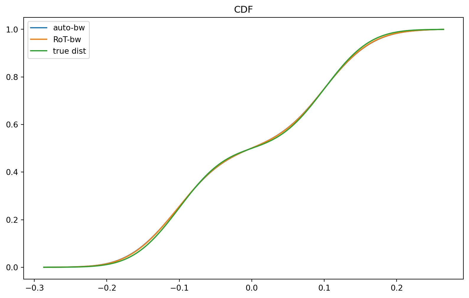
Relative Difference in CDF
Code
# Compute the relative difference
rel_diff_auto_cdf = np.abs(pdf_a / cdf_true - 1.0)
rel_diff_rot_cdf = np.abs(pdf_rot_a / cdf_true - 1.0)

# Plot the relative difference
plt.figure(figsize=(10, 6))
plt.title("CDF relative difference with respect to the true distribution")
plt.plot(x_a, rel_diff_auto_cdf, label="auto-bw")
plt.plot(x_a, rel_diff_rot_cdf, label="RoT-bw")
plt.grid()
plt.legend(loc="best")
plt.yscale("log")
plt.show()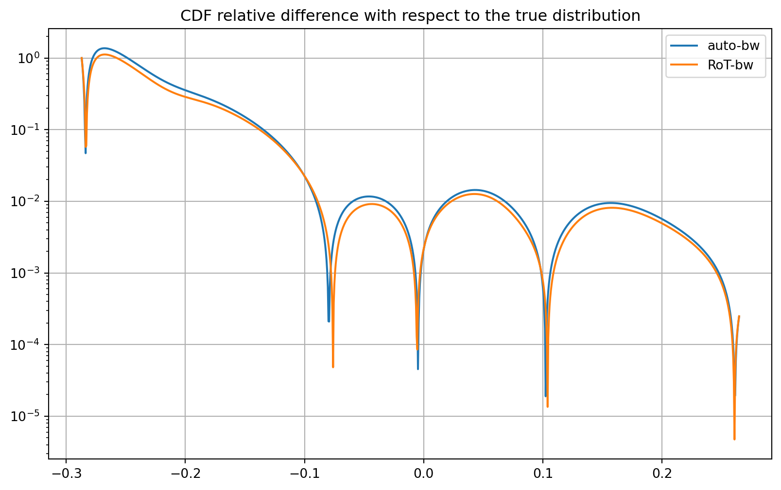
Inverse Cumulative Distribution Function (Inverse CDF)
Code
# Compute the inverse CDF for plotting
u_a = np.linspace(0, 1, 1000)
inv_pdf_a = [epdf.eval_inv_pdf(u) for u in u_a]
inv_pdf_rot_a = [epdf_rot.eval_inv_pdf(u) for u in u_a]

# Plot the inverse CDF
plt.figure(figsize=(10, 6))
plt.title("Inverse CDF")
plt.plot(u_a, inv_pdf_a, label="auto-bw")
plt.plot(u_a, inv_pdf_rot_a, label="RoT-bw")
plt.legend(loc="best")
plt.show()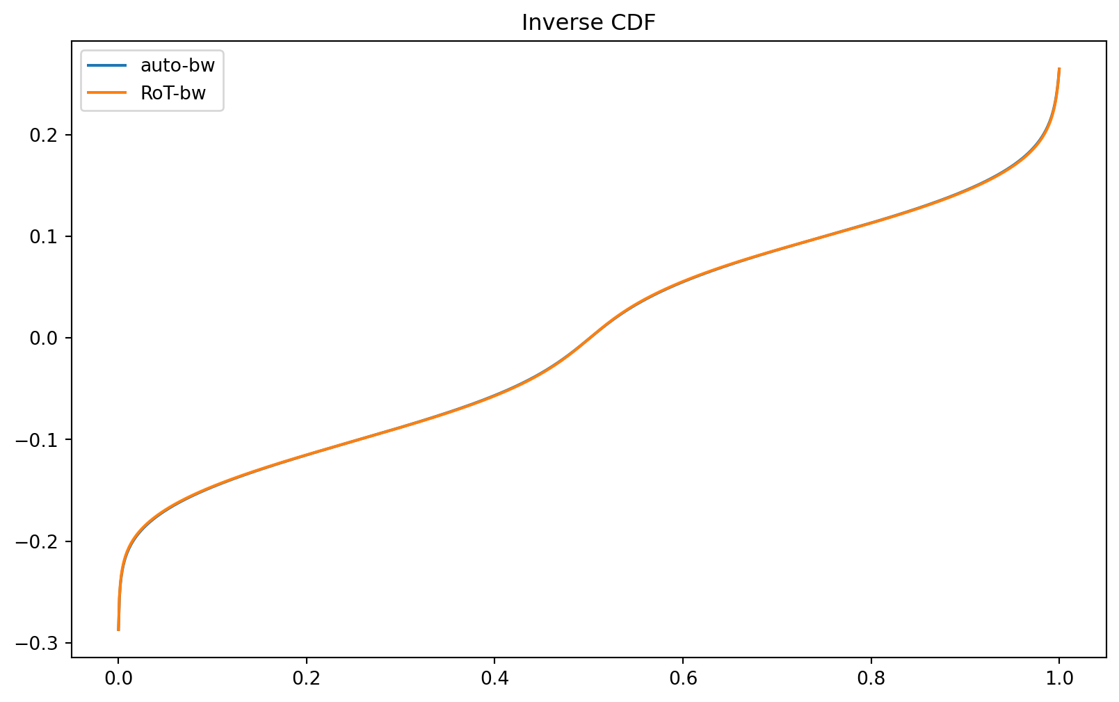
Conclusion
In this document, we demonstrated how to use the Ncm.StatsDist1dEPDF object from the numcosmo library to reconstruct the probability density function (PDF) and cumulative distribution function (CDF) of a distribution of points. We compared the results with the true distribution and visualized the differences. This example serves as a foundation for further exploration of empirical distribution functions in cosmological and statistical analyses.