import math
import numpy as np
import matplotlib.pyplot as plt

from numcosmo_py import Nc, Ncm

# Initialize the library
Ncm.cfg_init()Testing Power Spectra in Cosmological Models
Abstract
This document demonstrates how to test power spectra in cosmological models using the numcosmo library. It covers the setup of a cosmological model, computation of linear and nonlinear matter power spectra, and visualization of the results. The example compares the Eisenstein-Hu (EH) transfer function with the CLASS backend and includes HALOFIT for nonlinear corrections.
Introduction
This example demonstrates how to test power spectra in cosmological models using the numcosmo library. We will set up a cosmological model, compute the linear and nonlinear matter power spectra, and compare the results using the Eisenstein-Hu (EH) transfer function and the CLASS backend. The results are visualized to highlight the differences between the methods. This guide assumes familiarity with cosmological concepts and basic Python programming.
Prerequisites
Before running this example, make sure the numcosmo_py1 package is installed in your environment. If it is not already installed, follow the installation instructions in the NumCosmo documentation. In addition, we are using numpy and matplotlib for data manipulation and plotting. If you are using the conda installation, these packages are already installed.
1 NumCosmo is a C library for cosmology and astrophysics that uses GObject-Introspection to provide bindings for various programming languages. To improve the user interface, we provide a Python package, numcosmo_py. This package imports all NumCosmo bindings and includes additional helper functions to simplify library usage.
Import and Initialize
First, import the required modules and initialize the NumCosmo library. The Nc and Ncm modules provide the core functionality of the NumCosmo library. The call to Ncm.cfg_init() initializes the library objects.
Setting Up the Cosmological Model
We start by creating a new homogeneous and isotropic cosmological model (NcHICosmoDEXcdm) and setting its parameters. We also include a reionization model and a power-law primordial power spectrum.
# Create a new cosmological model with one massive neutrino
cosmo = Nc.HICosmoDEXcdm(massnu_length=1)
# Change the parameterization
cosmo.omega_x2omega_k()

cosmo["Omegak"] = 0.0
cosmo["w"] = -1.0
cosmo["Omegab"] = 0.04909244421
cosmo["Omegac"] = 0.26580755578
cosmo["massnu_0"] = 0.06
cosmo["ENnu"] = 2.0328

# Create a reionization model
reion = Nc.HIReionCamb.new()

# Create a power-law primordial power spectrum
prim = Nc.HIPrimPowerLaw.new()

# Set the Hubble constant
cosmo["H0"] = 67.31

# Set the primordial power spectrum parameters
prim["n_SA"] = 0.9658
prim["ln10e10ASA"] = 3.0904

# Set the reionization redshift
reion["z_re"] = 9.9999

# Add submodels to the cosmological model
cosmo.add_submodel(reion)
cosmo.add_submodel(prim)

# Print the model parameters
print("# Model parameters: ", end=" ")
cosmo.params_log_all()
print(f"# Omega_X0: {cosmo.E2Omega_de(0.0): 22.15g}")
# Model parameters: 67.31 0.26580755578 0 2.7245 0.24 2.0328 0.04909244421 -1 0.06 0.71611 0 1
# Omega_X0: 0.6836000217121Computing the Power Spectrum
We compute the linear matter power spectrum using both the Eisenstein-Hu (EH) transfer function and the CLASS backend. We also compute the nonlinear matter power spectrum using HALOFIT.
Linear Power Spectrum
# Create power spectrum objects
ps_cbe = Nc.PowspecMLCBE.new()  # CLASS backend
ps_eh = Nc.PowspecMLTransfer.new(Nc.TransferFuncEH.new())  # Eisenstein-Hu

# Set redshift and wavenumber bounds
z_min = 0.0
z_max = 2.0
nz = 5

k_min = 1.0e-5
k_max = 1.0e3

# Set the number of points for sampling
nk = 2000
nR = 2000
Rh8 = 8.0 / cosmo.h()

# Configure the power spectrum objects
ps_cbe.set_kmin(k_min)
ps_eh.set_kmin(k_min)

ps_cbe.set_kmax(k_max)
ps_eh.set_kmax(k_max)

ps_cbe.require_zi(z_min)
ps_cbe.require_zf(z_max)

ps_eh.require_zi(z_min)
ps_eh.require_zf(z_max)

# Prepare the power spectrum objects
ps_eh.prepare(cosmo)
ps_cbe.prepare(cosmo)

# Compute and plot the linear power spectrum
z_array = np.linspace(z_min, z_max, nz)
k_array = np.geomspace(k_min, k_max, nk)

Pk_cbe_a = np.array([ps_cbe.eval(cosmo, z, k) for z in z_array for k in k_array])
Pk_eh_a = np.array([ps_eh.eval(cosmo, z, k) for z in z_array for k in k_array])

Pk_cbe_a = np.reshape(Pk_cbe_a, (nz, nk))
Pk_eh_a = np.reshape(Pk_eh_a, (nz, nk))
The following code plots the linear power spectrum for different redshifts.
Code
plt.figure(figsize=(10, 6))

for i, z in enumerate(z_array):
    plt.plot(k_array, Pk_cbe_a[i, :], label=f"CLASS $z = {z:.2f}$")
    plt.plot(k_array, Pk_eh_a[i, :], label=f"EH    $z = {z:.2f}$")

plt.xlabel(r"$k \; [\mathrm{Mpc}^{-1}]$")
plt.ylabel(r"$k^3P(k, z)$")
plt.legend(loc="best")
plt.xscale("log")
plt.yscale("log")
plt.title("Linear Matter Power Spectrum")
plt.show()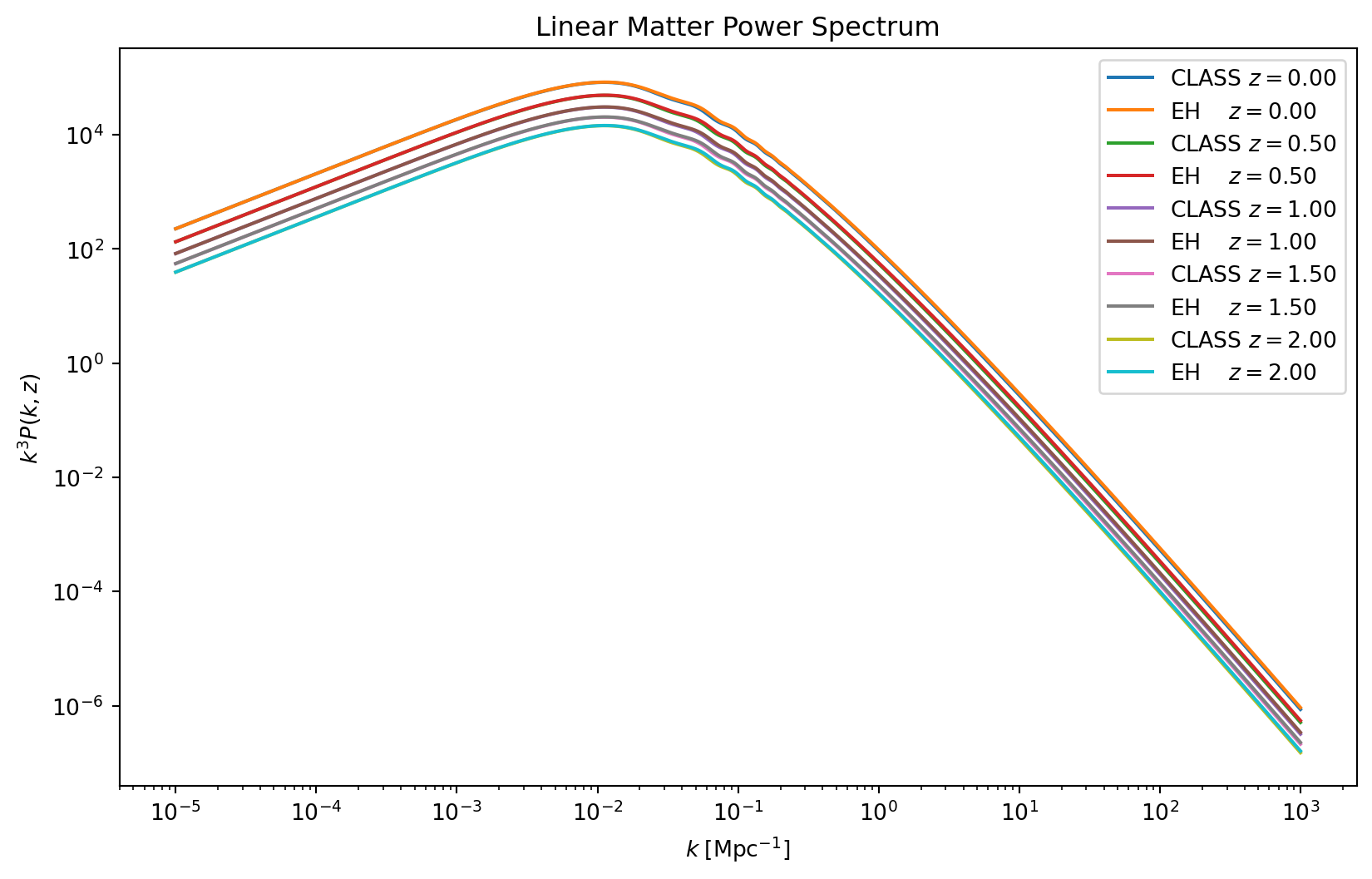
Relative Difference Between EH and CLASS
Code
plt.figure(figsize=(10, 6))

for i, z in enumerate(z_array):
    plt.plot(
        k_array, np.abs(1.0 - Pk_eh_a[i, :] / Pk_cbe_a[i, :]), label=f"$z = {z:.2f}$"
    )

plt.xlabel(r"$k \; [\mathrm{Mpc}^{-1}]$")
plt.ylabel(r"$1 - P_{EH}(k, z)/P_{CLASS}(k, z)$")
plt.legend(loc="best")
plt.xscale("log")
plt.yscale("log")
plt.title("Relative difference between the EH and CLASS PS")
plt.show()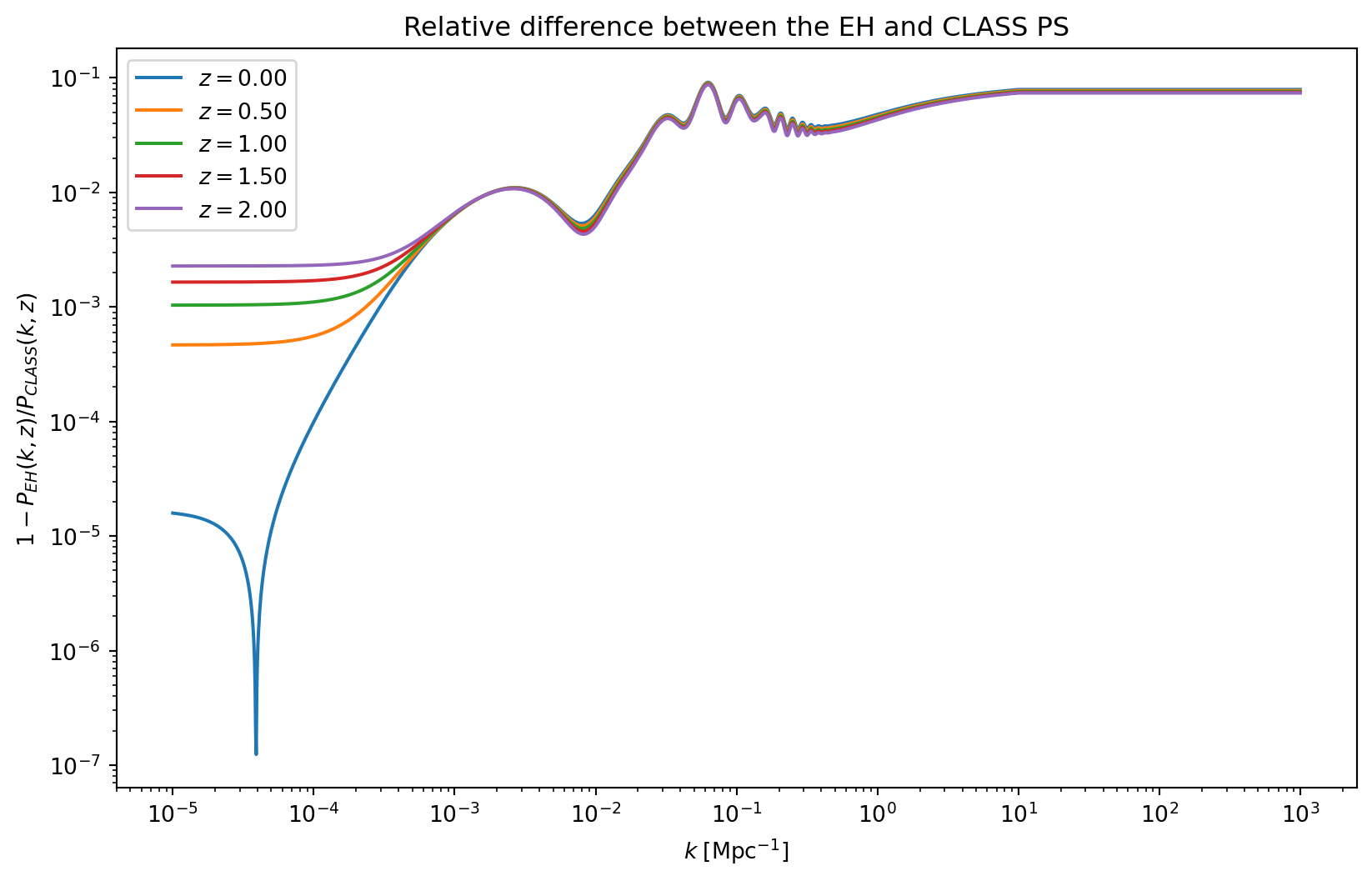
Nonlinear Power Spectrum with HALOFIT
Code
# Set up HALOFIT for nonlinear corrections
zmax_nl = 10.0
z_max = zmax_nl
pshf = Nc.PowspecMNLHaloFit.new(ps_cbe, zmax_nl, 1.0e-5)

pshf.set_kmin(k_min)
pshf.set_kmax(k_max)
pshf.require_zi(z_min)
pshf.require_zf(z_max)

pshf.prepare(cosmo)

# Compute and plot the nonlinear power spectrum
Pk_nl_cbe_a = np.array([pshf.eval(cosmo, z, k) for z in z_array for k in k_array])
Pk_nl_cbe_a = np.reshape(Pk_nl_cbe_a, (nz, nk))

# Plot the nonlinear power spectrum for different redshifts
plt.figure(figsize=(10, 6))

for i, z in enumerate(z_array):
    plt.plot(k_array, Pk_cbe_a[i, :], label=f"CLASS $z = {z:.2f}$")
    plt.plot(k_array, Pk_nl_cbe_a[i, :], label=f"CLASS+HaloFit $z = {z:.2f}$")

plt.xlabel(r"$k \; [\mathrm{Mpc}^{-1}]$")
plt.ylabel(r"$k^3 P(k, z)$")
plt.title("Linear and nonlinear matter power spectrum")
plt.legend(loc="best")
plt.xscale("log")
plt.yscale("log")
plt.show()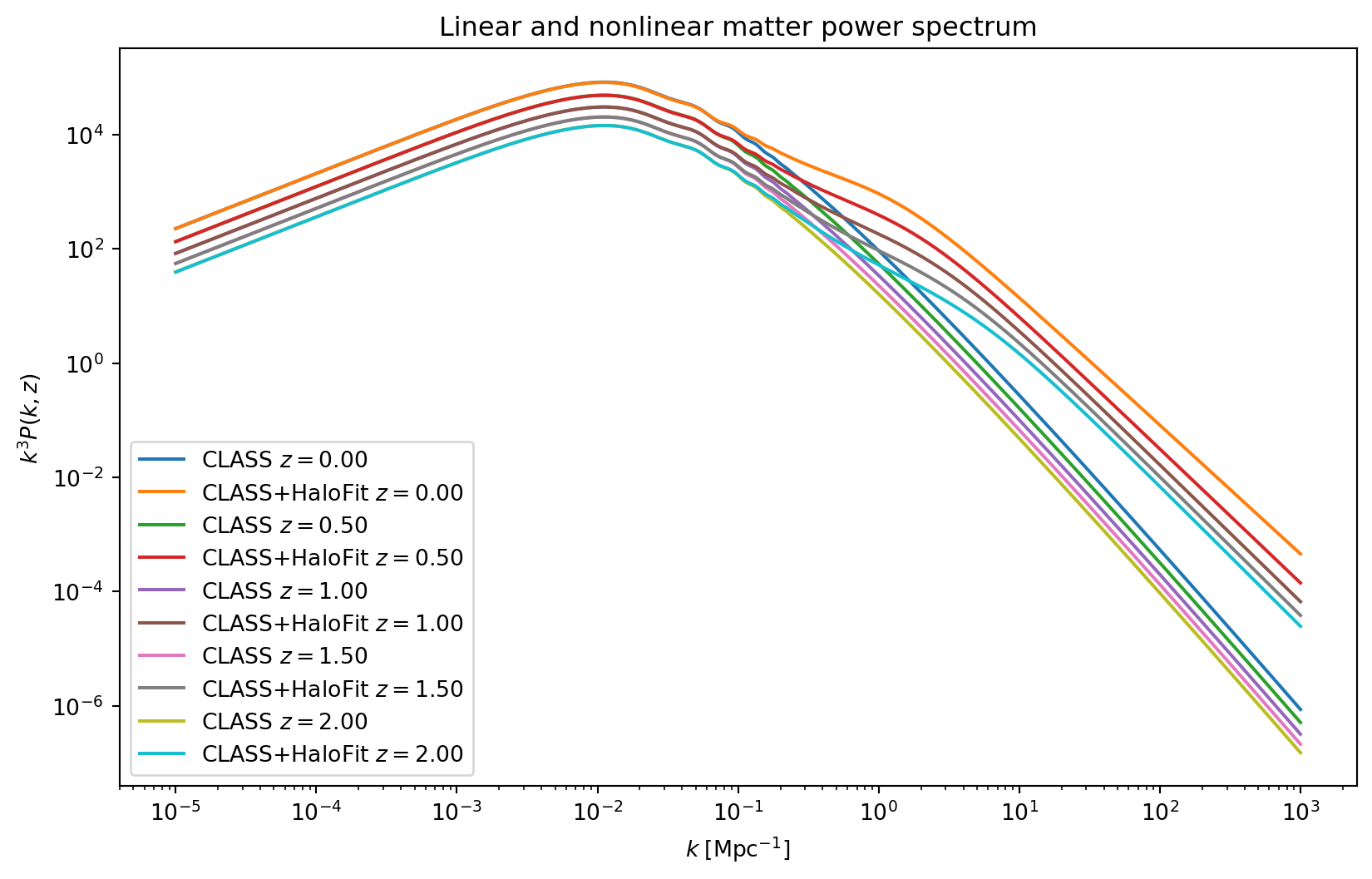
Conclusion
We computed the linear and nonlinear matter power spectra, compared the results using the Eisenstein-Hu transfer function and the CLASS backend, and visualized the differences. This example serves as a foundation for further exploration of power spectra in cosmological models.