import math
import numpy as np
import matplotlib.pyplot as plt

from numcosmo_py import Nc, Ncm

# Initialize the library
Ncm.cfg_init()Testing Tensor Modes in Primordial Models
Abstract
This document demonstrates how to test tensor modes in primordial cosmological models using the numcosmo library. It covers the setup of a cosmological model with tensor modes, computation of the power spectrum for different CMB observables (TT, TE, EE, BB), and visualization of the results.
Introduction
This example demonstrates how to test tensor modes in primordial cosmological models using the numcosmo library. We will create a cosmological model with tensor modes, compute the power spectrum for temperature (TT), temperature-polarization (TE), E-mode polarization (EE), and B-mode polarization (BB), and visualize the results. This guide assumes familiarity with cosmological concepts and basic Python programming.
Prerequisites
Before running this example, make sure the numcosmo_py1 package is installed in your environment. If it is not already installed, follow the installation instructions in the NumCosmo documentation. In addition, we are using numpy and matplotlib for data manipulation and plotting. If you are using the conda installation, these packages are already installed.
1 NumCosmo is a C library for cosmology and astrophysics that uses GObject-Introspection to provide bindings for various programming languages. To improve the user interface, we provide a Python package, numcosmo_py. This package imports all NumCosmo bindings and includes additional helper functions to simplify library usage.
Import and Initialize
First, import the required modules and initialize the NumCosmo library. The Nc and Ncm modules provide the core functionality of the NumCosmo library. The call to Ncm.cfg_init() initializes the library objects.
Setting Up the Primordial Model
We start by creating a new instance of the Nc.HIPrimPowerLaw model, which describes a power-law primordial power spectrum. We set the tensor-to-scalar ratio (r) and the tensor spectral index (n_T).
# Set the maximum multipole
lmax = 2500
# Create a new instance of HIPrimPowerLaw
prim = Nc.HIPrimPowerLaw.new()

# Set the tensor-to-scalar ratio and tensor spectral index
r = 1.0
prim.props.T_SA_ratio = r
prim.props.n_T = -1.0 * r / 8.0
Configuring the CLASS Backend
Next, we configure the CLASS backend to compute the power spectrum. We increase the precision for the primordial spectrum and set up the Boltzmann solver to include tensor modes.
# Create a new CLASS backend precision object
cbe_prec = Nc.CBEPrecision.new()
cbe_prec.props.k_per_decade_primordial = 50.0

# Create a new CLASS backend object with the specified precision
cbe = Nc.CBE.prec_new(cbe_prec)

# Create a new Boltzmann solver using the CLASS backend
Bcbe = Nc.HIPertBoltzmannCBE.full_new(cbe)

# Set the maximum multipole for the temperature power spectrum
Bcbe.set_TT_lmax(lmax)

# Enable tensor modes
Bcbe.set_tensor(True)

# Set the target Cl types (TT, TE, EE, BB)
Bcbe.append_target_Cls(Nc.DataCMBDataType.TT)
Bcbe.append_target_Cls(Nc.DataCMBDataType.TE)
Bcbe.append_target_Cls(Nc.DataCMBDataType.EE)
Bcbe.append_target_Cls(Nc.DataCMBDataType.BB)

# Set the maximum multipole for each Cl type
Bcbe.set_TT_lmax(lmax)
Bcbe.set_TE_lmax(lmax)
Bcbe.set_EE_lmax(lmax)
Bcbe.set_BB_lmax(30)
Setting Up the Cosmological Model
We create a new homogeneous and isotropic cosmological model (NcHICosmoDEXcdm) and add the primordial and reionization submodels.
# Create a new cosmological model
cosmo = Nc.HICosmoDEXcdm.new()
cosmo.omega_x2omega_k()
cosmo.param_set_by_name("Omegak", 0.0)

# Create a new reionization object
reion = Nc.HIReionCamb.new()

# Add submodels to the cosmological model
cosmo.add_submodel(reion)
cosmo.add_submodel(prim)
Computing the Power Spectrum
We compute the power spectrum with contributions from both scalar and tensor modes and compare with the power spectrum without the tensor contribution.
# Prepare the Boltzmann solver with the cosmological model
Bcbe.prepare(cosmo)

# Create vectors to store the computed Cl's
Cls1_TT = Ncm.Vector.new(lmax + 1)
Cls1_TE = Ncm.Vector.new(lmax + 1)
Cls1_EE = Ncm.Vector.new(lmax + 1)
Cls1_BB = Ncm.Vector.new(31)

# Compute the Cl's with tensor contribution
Bcbe.get_TT_Cls(Cls1_TT)
Bcbe.get_TE_Cls(Cls1_TE)
Bcbe.get_EE_Cls(Cls1_EE)
Bcbe.get_BB_Cls(Cls1_BB)

# Compute the Cl's without tensor contribution
prim.props.T_SA_ratio = 1.0e-30
Bcbe.prepare(cosmo)

Cls2_TT = Ncm.Vector.new(lmax + 1)
Cls2_TE = Ncm.Vector.new(lmax + 1)
Cls2_EE = Ncm.Vector.new(lmax + 1)
Cls2_BB = Ncm.Vector.new(31)

Bcbe.get_TT_Cls(Cls2_TT)
Bcbe.get_TE_Cls(Cls2_TE)
Bcbe.get_EE_Cls(Cls2_EE)
Bcbe.get_BB_Cls(Cls2_BB)
Processing and Plotting the Results
We process the computed \(C_\ell\)’s and plot the results to compare the tensor and scalar contributions.
# Convert the computed Cl's to numpy arrays
Cls1_TT_a = Cls1_TT.dup_array()
Cls1_TE_a = Cls1_TE.dup_array()
Cls1_EE_a = Cls1_EE.dup_array()
Cls1_BB_a = Cls1_BB.dup_array()

Cls2_TT_a = Cls2_TT.dup_array()
Cls2_TE_a = Cls2_TE.dup_array()
Cls2_EE_a = Cls2_EE.dup_array()
Cls2_BB_a = Cls2_BB.dup_array()

# Create arrays of multipoles
ell = np.array(list(range(2, lmax + 1)))
ell_BB = np.array(list(range(2, 31)))

# Scale the Cl's by ell(ell+1) for better visualization
Cls1_TT_a = ell * (ell + 1.0) * np.array(Cls1_TT_a[2:])
Cls1_TE_a = ell * (ell + 1.0) * np.array(Cls1_TE_a[2:])
Cls1_EE_a = ell * (ell + 1.0) * np.array(Cls1_EE_a[2:])
Cls1_BB_a = ell_BB * (ell_BB + 1.0) * np.array(Cls1_BB_a[2:])

Cls2_TT_a = ell * (ell + 1.0) * np.array(Cls2_TT_a[2:])
Cls2_TE_a = ell * (ell + 1.0) * np.array(Cls2_TE_a[2:])
Cls2_EE_a = ell * (ell + 1.0) * np.array(Cls2_EE_a[2:])
Cls2_BB_a = ell_BB * (ell_BB + 1.0) * np.array(Cls2_BB_a[2:])
Plotting the Results
We plot the power spectra for TT, TE, EE, and BB modes to compare the tensor and scalar contributions.
Code
plt.figure(figsize=(10, 6))
plt.title(r"With and without tensor contribution to $C_\ell^\mathrm{TT}$")
plt.plot(ell[:28], Cls1_TT_a[:28], "r", label="Tensor")
plt.plot(ell[:28], Cls2_TT_a[:28], "b--", label="Scalar")
plt.xlabel(r"$\ell$")
plt.ylabel(r"$\ell(\ell+1)C_\ell$")
plt.legend(loc="best")
plt.show()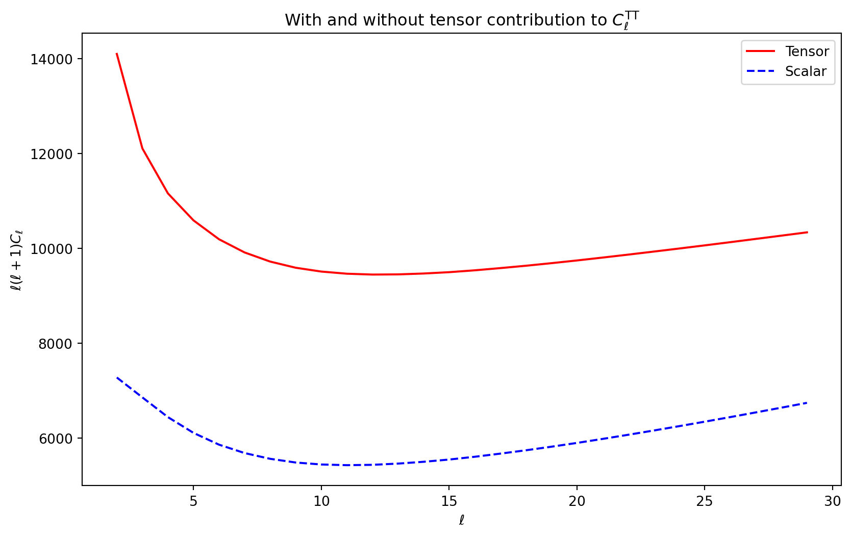
Code
plt.figure(figsize=(10, 6))
plt.title(r"With and without tensor contribution to $C_\ell^\mathrm{TE}$")
plt.plot(ell[:28], Cls1_TE_a[:28], "r", label="Tensor")
plt.plot(ell[:28], Cls2_TE_a[:28], "b--", label="Scalar")
plt.xlabel(r"$\ell$")
plt.ylabel(r"$\ell(\ell+1)C_\ell$")
plt.legend(loc="best")
plt.show()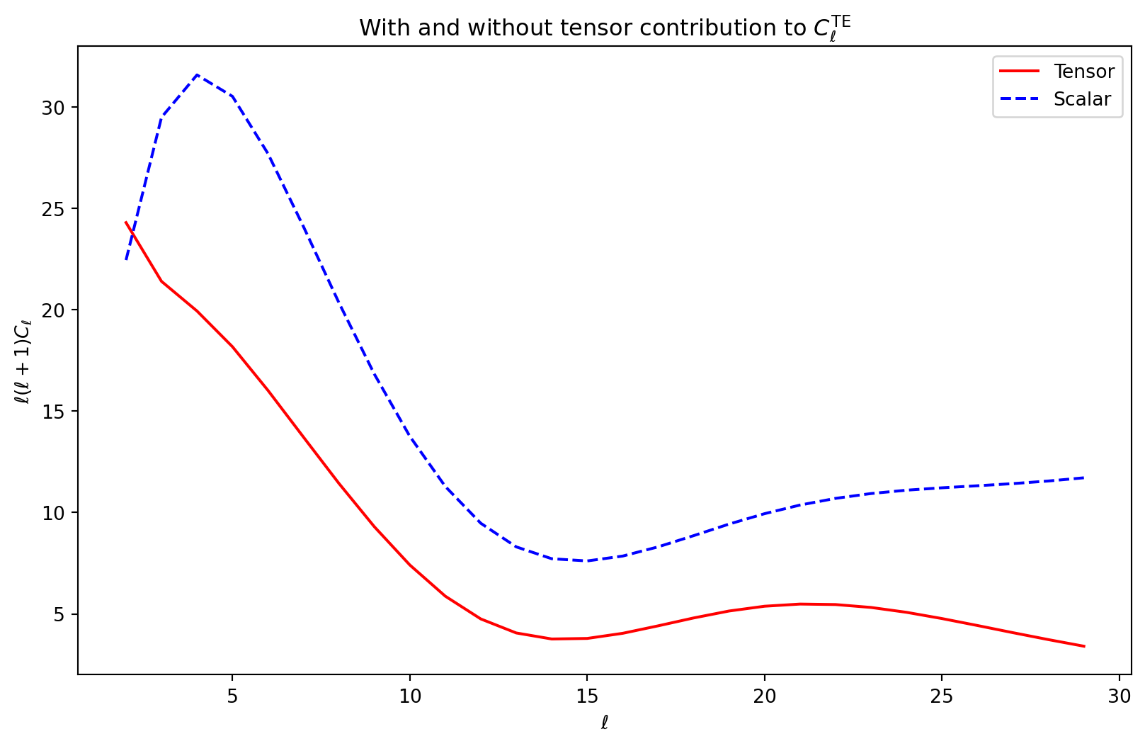
Code
plt.figure(figsize=(10, 6))
plt.title(r"With and without tensor contribution to $C_\ell^\mathrm{EE}$")
plt.plot(ell[:28], Cls1_EE_a[:28], "r", label="Tensor")
plt.plot(ell[:28], Cls2_EE_a[:28], "b--", label="Scalar")
plt.xlabel(r"$\ell$")
plt.ylabel(r"$\ell(\ell+1)C_\ell$")
plt.legend(loc="best")
plt.show()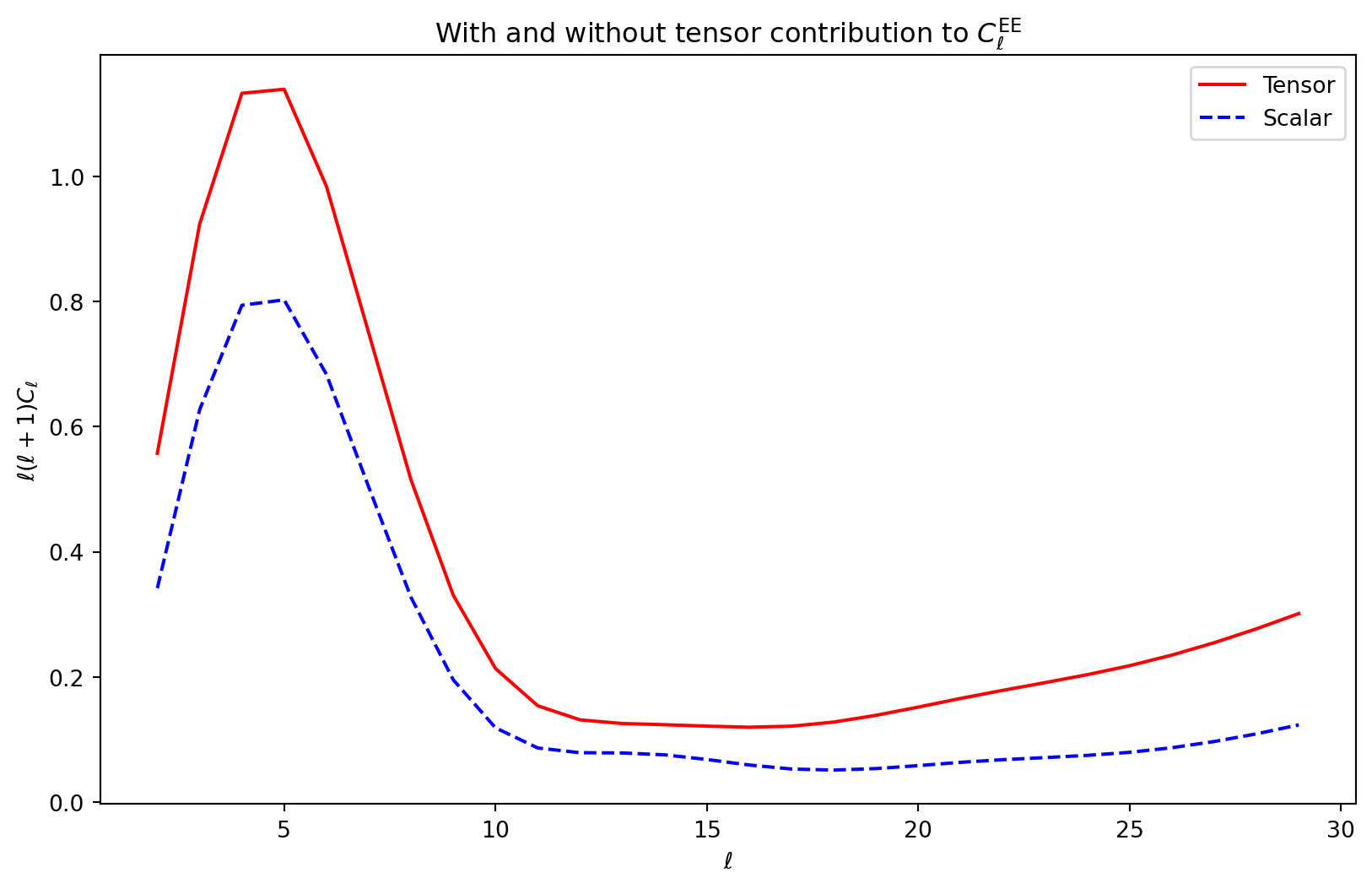
Code
plt.figure(figsize=(10, 6))
plt.title(r"With and without tensor contribution to $C_\ell^\mathrm{BB}$")
plt.plot(ell_BB[:28], Cls1_BB_a[:28], "r", label="Tensor")
plt.plot(ell_BB[:28], Cls2_BB_a[:28], "b--", label="Scalar")
plt.xlabel(r"$\ell$")
plt.ylabel(r"$\ell(\ell+1)C_\ell$")
plt.legend(loc="best")
plt.show()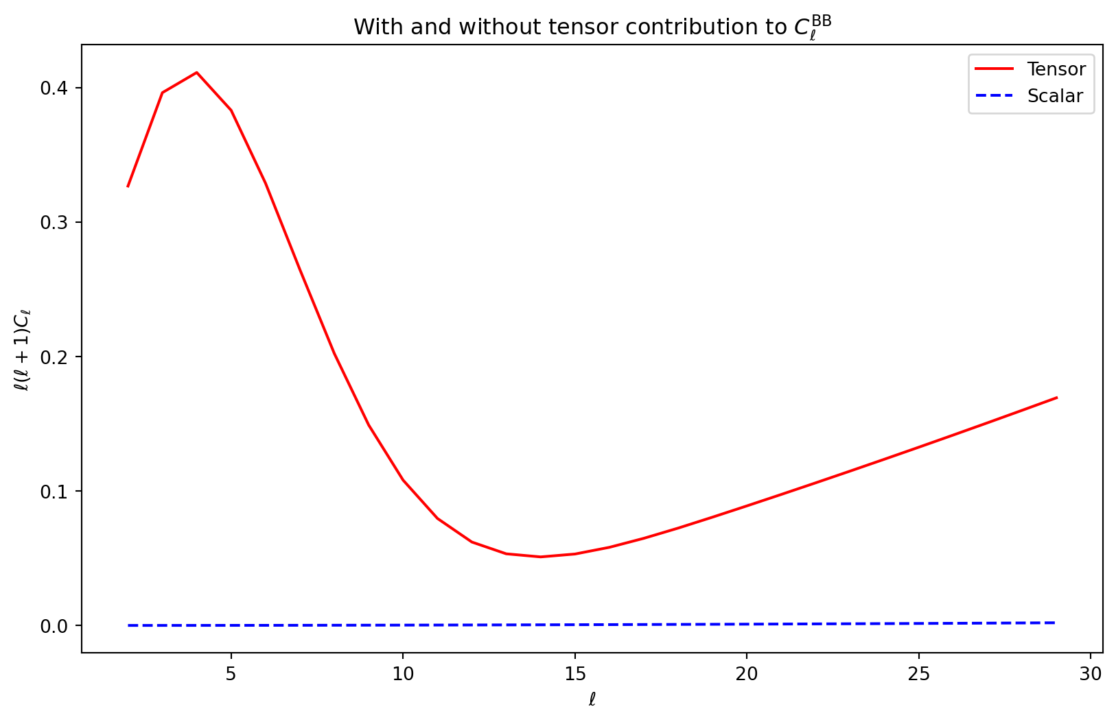
Conclusion
In this document, we demonstrated how to test tensor modes in primordial cosmological models using the numcosmo library. We computed the power spectrum for TT, TE, EE, and BB modes, comparing the contributions of tensor and scalar modes. The results were visualized to highlight the impact of tensor modes on the CMB power spectra.