def doc_theme():
    return theme_minimal() + theme(
        panel_grid_minor=element_line(color="gray", linetype="--"),
)Supernova Type Ia Analysis
Introduction
In this example, we demonstrate how to use NumCosmo to compute cosmological observables and fit a model to data. We use the numcosmo_py1 package to simplify the library usage and plotnine for data visualization.
1 NumCosmo is a C library for cosmology and astrophysics that uses GObject-Introspection to provide bindings for various programming languages. To improve the user interface, we provide a Python package, numcosmo_py. This package imports all NumCosmo bindings and includes additional helper functions to simplify library usage.
Computational Cosmology
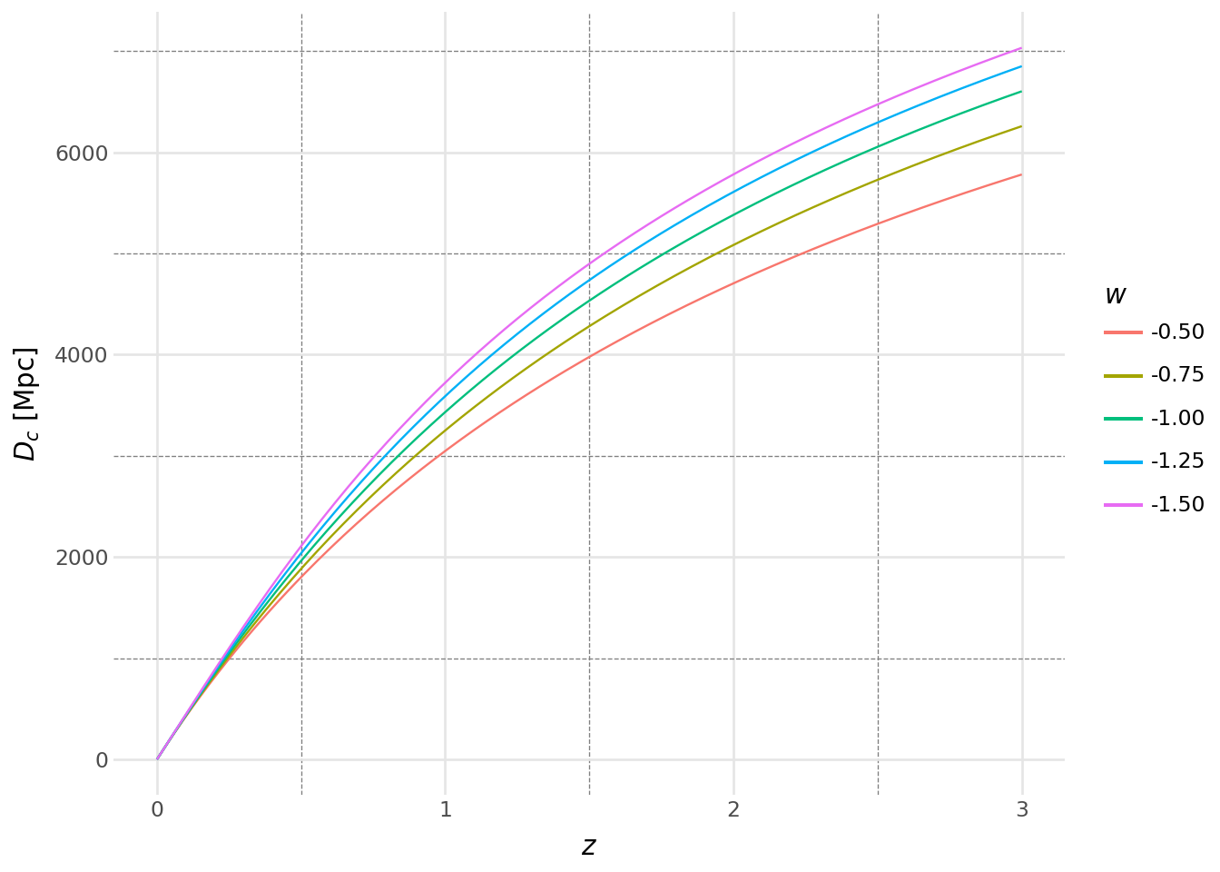
NumCosmo provides tools for calculating cosmological observables with precision. For example, the comoving distance in an XCDM cosmology up to a redshift of \(z = 3.0\) can be computed with a few lines of code using the parameters \(\Omega_{c0} = 0.25\), \(\Omega_{b0} = 0.05\), and \(w\) varying from \(-1.5\) to \(-0.5\).
import numpy as np
import pandas as pd
from plotnine import *

# This modules must be loaded before getdist to avoid getdist's secondary effects
import numcosmo_py.plotting
import getdist
from getdist import plots

from numcosmo_py import Nc, Ncm
from numcosmo_py.plotting import mcat_to_catalog_data

# Initialize the library
Ncm.cfg_init()

cosmo = Nc.HICosmoDEXcdm()
dist = Nc.Distance()

cosmo["Omegac"] = 0.25
cosmo["Omegab"] = 0.05

dist_pd_a = []
for w in np.linspace(-1.5, -0.5, 5):
    cosmo["w"] = w
    dist.prepare(cosmo)
    RH_Mpc = cosmo.RH_Mpc()

    z_a = np.linspace(0.0, 3.0, 200)
    d_a = np.array([dist.comoving(cosmo, z) for z in z_a]) * RH_Mpc

    dist_pd_a.append(pd.DataFrame({"z": z_a, "Dc": d_a, "eos_w": f"{w: .2f}"}))

dist_pd = pd.concat(dist_pd_a)
The code above computes the comoving distance for an XCDM cosmology with different values of the equation of state parameter \(w\).
Code
(
    ggplot(dist_pd, aes("z", "Dc", color="eos_w"))
    + geom_line()
    + labs(x=r"$z$", y=r"$D_c$ [Mpc]", color=r"$w$")
    + doc_theme()
)
The Modeling
NumCosmo’s computational objects are designed for direct use in statistical analyses. In the example above, the HICosmoDEXcdm class defines the cosmological model, which is a subclass of the HICosmo class representing a homogeneous isotropic cosmology. The model’s parameters can be accessed and managed within a model set, using the MSet class, which serves as the main container for all models in a given analysis.
mset = Ncm.MSet.new_array([cosmo])
mset.pretty_log()
#----------------------------------------------------------------------------------
# Model[03000]:
# - NcHICosmo : XCDM - Constant EOS
#----------------------------------------------------------------------------------
# Model parameters
# - H0[00]: 67.36 [FIXED]
# - Omegac[01]: 0.25 [FIXED]
# - Omegax[02]: 0.7 [FIXED]
# - Tgamma0[03]: 2.7245 [FIXED]
# - Yp[04]: 0.24 [FIXED]
# - ENnu[05]: 3.046 [FIXED]
# - Omegab[06]: 0.05 [FIXED]
# - w[07]: -0.5 [FIXED]Fitting Model to Data
Once models are defined and the free parameters are set, they can be analyzed using a variety of statistical methods. For example, the best-fit parameters for a given model can be found by maximizing the likelihood function.
Code
cosmo.props.w_fit = True
cosmo.props.Omegac_fit = True
mset.prepare_fparam_map()

lh = Ncm.Likelihood(
    dataset=Ncm.Dataset.new_array(
        [Nc.DataDistMu.new_from_id(dist, Nc.DataSNIAId.SIMPLE_UNION2_1)]
    )
)
fit = Ncm.Fit.factory(
    Ncm.FitType.NLOPT, "ln-neldermead", lh, mset, Ncm.FitGradType.NUMDIFF_FORWARD
)
fit.run(Ncm.FitRunMsgs.SIMPLE)
fit.log_info()
fit.fisher()
fit.log_covar()
#----------------------------------------------------------------------------------
# Model fitting. Iterating using:
# - solver: NLOpt:ln-neldermead
# - differentiation: Numerical differentiation (forward)
#................
# Minimum found with precision: |df|/f = 1.00000e-08 and |dx| = 1.00000e-05
# Elapsed time: 00 days, 00:00:00.7900860
# iteration [000076]
# function evaluations [000078]
# gradient evaluations [000000]
# degrees of freedom [000577]
# m2lnL = -237.488027238987 ( -237.48803 )
# Fit parameters:
# 0.230549141552248 -1.02976361340715
#----------------------------------------------------------------------------------
# Data used:
# - Union2.1 sample
#----------------------------------------------------------------------------------
# Model[03000]:
# - NcHICosmo : XCDM - Constant EOS
#----------------------------------------------------------------------------------
# Model parameters
# - H0[00]: 67.36 [FIXED]
# - Omegac[01]: 0.230549141552248 [FREE]
# - Omegax[02]: 0.7 [FIXED]
# - Tgamma0[03]: 2.7245 [FIXED]
# - Yp[04]: 0.24 [FIXED]
# - ENnu[05]: 3.046 [FIXED]
# - Omegab[06]: 0.05 [FIXED]
# - w[07]: -1.02976361340715 [FREE]
#----------------------------------------------------------------------------------
# NcmMSet parameters covariance matrix
# -------------------------------
# Omegac[03000:01] = 0.2305 +/- 0.06232 | 1 | -0.9297 |
# w[03000:07] = -1.03 +/- 0.08595 | -0.9297 | 1 |
# -------------------------------The code above fits the XCDM model to the Union2.1 dataset, which contains supernova type Ia data. It computes the best-fit parameters for the model and the covariance matrix of the parameters using the Fisher matrix.
lhr2d = Ncm.LHRatio2d.new(
fit,
mset.fparam_get_pi_by_name("Omegac"),
mset.fparam_get_pi_by_name("w"),
1.0e-3,
)
best_fit = pd.DataFrame(
{
"Omegac": [cosmo.props.Omegac],
"w": [cosmo.props.w],
"sigma": "Best-fit",
"region": "Best-fit",
}
)
regions_pd_list = []
for i, sigma in enumerate(
[Ncm.C.stats_1sigma(), Ncm.C.stats_2sigma(), Ncm.C.stats_3sigma()]
):
fisher_rg = lhr2d.fisher_border(sigma, 300.0, Ncm.FitRunMsgs.NONE)
Omegac_a = np.array(fisher_rg.p1.dup_array())
w_a = np.array(fisher_rg.p2.dup_array())
regions_pd_list.append(
pd.DataFrame(
{
"Omegac": Omegac_a,
"w": w_a,
"sigma": rf"{i+1}$\sigma$",
"region": "Fisher",
}
)
)
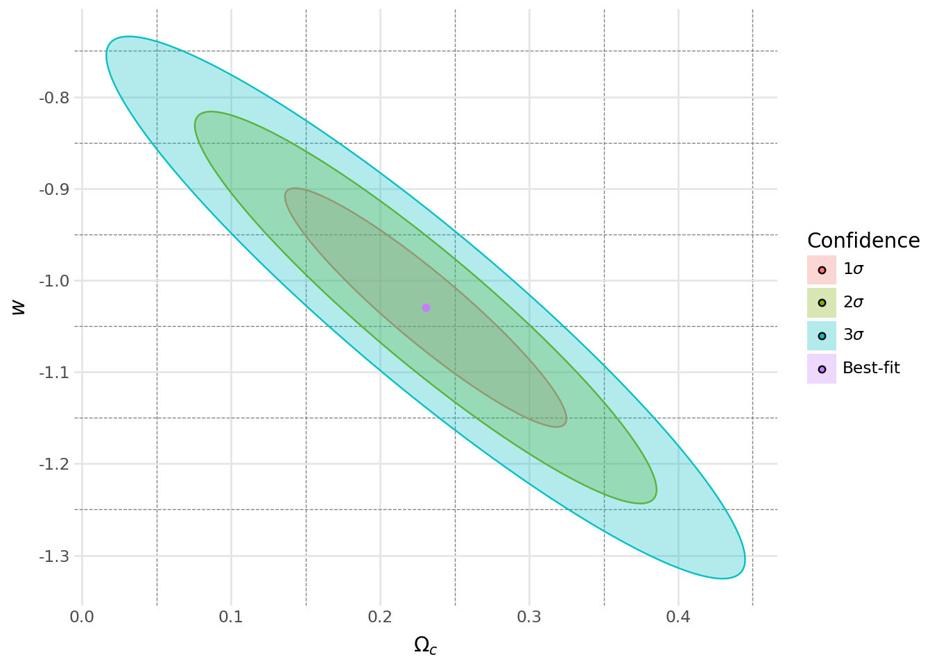
regions_pd = pd.concat(regions_pd_list)The code above computes the confidence regions for the best-fit parameters using the Fisher matrix.
Code
(
    ggplot(regions_pd, aes("Omegac", "w", fill="sigma", color="sigma"))
    + geom_polygon(alpha=0.3)
    + geom_point(data=best_fit)
    + labs(x=r"$\Omega_c$", y=r"$w$", fill=r"Confidence")
    + guides(fill=guide_legend(), color=False)
    + doc_theme()
)
Running a MCMC Analysis
NumCosmo also provides tools for running Markov Chain Monte Carlo (MCMC) analyses. The code below runs an MCMC analysis using the APES algorithm.
init_sampler = Ncm.MSetTransKernGauss.new(0)
init_sampler.set_mset(mset)
init_sampler.set_prior_from_mset()
init_sampler.set_cov(fit.get_covar())
nwalkers = 300
walker = Ncm.FitESMCMCWalkerAPES.new(nwalkers, mset.fparams_len())
esmcmc = Ncm.FitESMCMC.new(fit, nwalkers, init_sampler, walker, Ncm.FitRunMsgs.NONE)
esmcmc.start_run()
esmcmc.run(6)
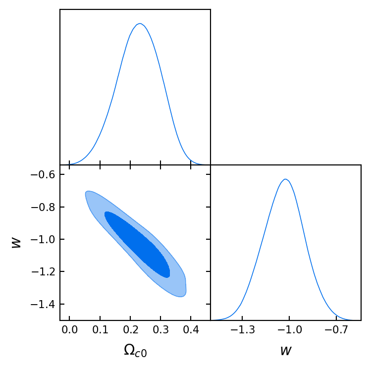
esmcmc.end_run()Finally, we can extract the MCMC samples and visualize the results.
mcat = esmcmc.peek_catalog()
mcat.trim(2, 1)

cd = mcat_to_catalog_data(mcat, name="XCDM Supernova Ia Analysis")

g = plots.get_subplot_plotter()
g.triangle_plot(cd.to_mcsamples(), shaded=False, filled=True)
Removed no burn in