import math
from numcosmo_py import Nc, Ncm
from numcosmo_py.helper import register_model_class
import numpy as np
import matplotlib.pyplot as plt

Ncm.cfg_init()Implementing a Primordial Cosmology Model
Introduction
This example demonstrates how to implement a primordial cosmology model using the numcosmo library. In this example, we create a primordial cosmological model and compute comoving distances for a range of redshifts.
Prerequisites
Before running this example, make sure the numcosmo_py1 package is installed in your environment. If it is not already installed, follow the installation instructions in the NumCosmo documentation. In addition, we are using numpy, matplotlib and pandas for data manipulation and plotting. If you are using the conda installation, these packages are already installed.
1 NumCosmo is a C library for cosmology and astrophysics that uses GObject-Introspection to provide bindings for various programming languages. To improve the user interface, we provide a Python package, numcosmo_py. This package imports all NumCosmo bindings and includes additional helper functions to simplify library usage.
Import and Initialize
First, import the required modules and initialize the NumCosmo library. We also import numpy and matplotlib. The Nc and Ncm modules provide the core functionality of the NumCosmo library. The call to Ncm.cfg_init() initializes the library objects.
Creating a Primordial Cosmological Model
To create a primordial cosmological model (NcHIPrimExample), we need to define a new class that inherits from the NcHIPrim abstract class. This process involves using the NcmModelBuilder class to construct the model and register it within the GObject type system. Below, we outline the steps to achieve this.
Step 1: Define the Model Using NcmModelBuilder
We start by creating a new NcmModelBuilder object, which allows us to define a new model (NcHIPrimExample) that implements the NcHIPrim abstract class. The NcmModelBuilder class provides a convenient way to define models and their parameters.
# Create a new ModelBuilder object for the NcHIPrimExample model
mb = Ncm.ModelBuilder.new(Nc.HIPrim, "NcHIPrimExample", "An example primordial model")
Step 2: Add Parameters to the Model
Next, we add parameters to the model. These parameters will be used in statistical analyses and simulations. Here, we define the following parameters:
A_s: The amplitude of the primordial power spectrum. This parameter controls the overall amplitude of the power spectrum.n_s: The spectral index, which describes the slope of the primordial power spectrum.a,b, andc: Additional parameters to describe modifications to the primordial spectrum.
# Add the amplitude parameter A_s
mb.add_sparam("A_s", "As", 0.0, 1.0, 0.1, 0.0, 1.0e-9, Ncm.ParamType.FREE)

# Add the spectral index parameter n_s
mb.add_sparam("n_s", "ns", 0.5, 1.5, 0.1, 0.0, 0.96, Ncm.ParamType.FREE)

# Add additional parameters for spectrum modifications
mb.add_sparam("a", "a", 0.0, 1.0, 0.01, 0.0, 0.5, Ncm.ParamType.FREE)
mb.add_sparam("b", "b", 0.0, 1.0e4, 0.10, 0.0, 100.0, Ncm.ParamType.FREE)
mb.add_sparam("c", "c", 0.0, 6.0, 0.10, 0.0, 0.0, Ncm.ParamType.FREE)
Step 3: Register the Model Class
Once the parameters are defined, we register the model class using the register_model_class function. This step finalizes the creation of the NcHIPrimExample class, which is now a subclass of NcHIPrim with the specified parameters.
# Register the model class
HIPrimExample = register_model_class(mb)
At this point, HIPrimExample is a fully defined subclass of NcHIPrim with the parameters A_s, n_s, a, b, and c. However, to make the model functional, we need to implement the NcHIPrim interface by subclassing HIPrimExample and providing the necessary methods.
Implementing the NcHIPrim Interface
To complete the model, we need to subclass HIPrimExample and implement the methods required by the NcHIPrim interface. This involves defining how the primordial power spectrum is calculated based on the model’s parameters. Below is an outline of the steps required:
- Subclass
HIPrimExample: Create a new class that inherits fromHIPrimExample. - Implement Required Methods: Define methods such as
do_lnSA_powspec_lnkto compute the primordial power spectrum.
Note that it is not necessary to register the model class again after implementing the interface.
Here’s an example implementation:
class HIPrimExampleImpl(HIPrimExample):
    """Example implementation of a primordial cosmology model."""

    def do_lnSA_powspec_lnk(self, lnk: float) -> float:
        """
        Return the natural logarithm of the adiabatic power spectrum at a given ln(k).

        :param lnk: The natural logarithm of the wavenumber k.

        :return: The natural logarithm of the power spectrum at ln(k).
        """
        lnk0 = self.get_lnk_pivot()  # Get the pivot wavenumber
        lnka = lnk - lnk0  # Normalize ln(k) with respect to the pivot
        ka = math.exp(lnka)  # Convert ln(k) to k
        As = self.props.As  # Amplitude parameter
        ns = self.props.ns  # Spectral index parameter
        a = self.props.a  # Spectrum modification parameter
        b = self.props.b  # Spectrum modification parameter
        c = self.props.c  # Spectrum modification parameter
        a2 = a * a  # Precompute a^2 for efficiency

        # Compute the power spectrum
        return (
            (ns - 1.0) * lnka
            + math.log(As)
            + math.log1p(a2 * math.cos(b * ka + c) ** 2)
        )

    def get_lnSA_powspec_lnk0(self) -> float:
        """
        Return the natural logarithm of the adiabatic power spectrum at the pivot wavenumber.

        :return: The natural logarithm of the power spectrum at the pivot wavenumber.
        """
        As = self.props.As  # Amplitude parameter
        a = self.props.a  # Spectrum modification parameter
        b = self.props.b  # Spectrum modification parameter
        c = self.props.c  # Spectrum modification parameter
        a2 = a * a  # Precompute a^2 for efficiency

        # Compute the power spectrum at the pivot wavenumber
        return math.log(As) + math.log1p(a2 * math.cos(b + c) ** 2)
Explanation of the Implementation
do_lnSA_powspec_lnkMethod: This method computes the natural logarithm of the primordial power spectrum for the adiabatic scalar mode at a given wavenumberk. It uses the model’s parameters (As,ns,a,b, andc) to calculate the spectrum. The final expression for the power spectrum is: \[ \ln P(k) = (n_s - 1) \ln k + \ln A_s + \ln \left[1 + a^2 \cos^2\left(b \frac{k}{k_0} + c\right)\right], \] wherek_0is the pivot wavenumber.get_lnSA_powspec_lnk0Method: This method computes the natural logarithm of the power spectrum at the pivot wavenumber, which is a reference point for cosmological calculations.- Parameter Retrieval: The
self.propsattribute is used to access the model’s parameters. - Power Spectrum Calculation: The power spectrum is computed using a combination of the parameters and the wavenumber
k.
With this implementation, the NcHIPrimExample model is now fully functional and ready for use in cosmological simulations and analyses.
Computing the Power Spectrum
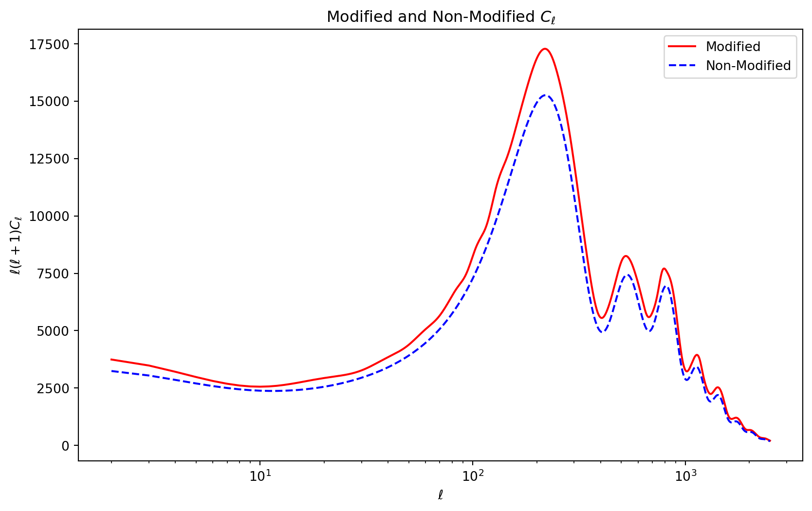
In this section, we demonstrate how to use the HIPrimExampleImpl model to compute the power spectrum and compare it with a non-modified spectrum. The following Python code sets up the cosmological model, computes the power spectrum, and generates a plot.
Set Up
# Maximum multipole for the power spectrum calculation
lmax = 2500
# Create a new instance of the primordial model
prim = HIPrimExampleImpl()

# Print the model parameters
print(f"# As        = {prim.props.As}")
print(f"# P (k = 1) = {prim.SA_powspec_k(1.0)}")
print(f"# (a, b, c) = ({prim.props.a}, {prim.props.b}, {prim.props.c})")
# As = 1e-09
# P (k = 1) = 9.170164114354885e-10
# (a, b, c) = (0.5, 100.0, 0.0)Configure the CLASS Backend
# Create a new CLASS backend precision object
cbe_prec = Nc.CBEPrecision.new()

# Increase k_per_decade_primordial for better resolution
cbe_prec.props.k_per_decade_primordial = 50.0

# Disable tight coupling approximation for higher accuracy
cbe_prec.props.tight_coupling_approximation = 0

# Create a new CLASS backend object with the specified precision
cbe = Nc.CBE.prec_new(cbe_prec)
Set Up the Boltzmann Solver
# Create a new Boltzmann solver using the CLASS backend
Bcbe = Nc.HIPertBoltzmannCBE.full_new(cbe)

# Set the maximum multipole for the temperature power spectrum
Bcbe.set_TT_lmax(lmax)

# Specify which CMB data to use (TT spectrum in this case)
Bcbe.set_target_Cls(Nc.DataCMBDataType.TT)

# Enable the use of lensed Cl's
Bcbe.set_lensed_Cls(True)
Set Up the Cosmological Model
# Create a new homogeneous and isotropic cosmological model (NcHICosmoDEXcdm)
cosmo = Nc.HICosmoDEXcdm.new()

# Convert curvature density parameter to omega_k
cosmo.omega_x2omega_k()

# Set the curvature density parameter to zero (flat universe)
cosmo.param_set_by_name("Omegak", 0.0)

# Create a new reionization object
reion = Nc.HIReionCamb.new()

# Add submodels (reionization and primordial spectrum) to the cosmological model
cosmo.add_submodel(reion)
cosmo.add_submodel(prim)
Compute the Power Spectrum
# Prepare the Boltzmann solver with the cosmological model
Bcbe.prepare(cosmo)

# Create vectors to store the computed Cl's
Cls1 = Ncm.Vector.new(lmax + 1)
Cls2 = Ncm.Vector.new(lmax + 1)

# Compute the temperature power spectrum with the modified primordial spectrum
Bcbe.get_TT_Cls(Cls1)

# Disable the modification (set a = 0) and recompute the power spectrum
prim.props.a = 0
Bcbe.prepare(cosmo)
Bcbe.get_TT_Cls(Cls2)

# Convert the computed Cl's to numpy arrays for plotting
Cls1_a = np.array(Cls1.dup_array())
Cls2_a = np.array(Cls2.dup_array())

# Remove the first two multipoles (monopole and dipole)
Cls1_a = np.array(Cls1_a[2:])
Cls2_a = np.array(Cls2_a[2:])

# Create an array of multipoles for plotting
ell = np.array(list(range(2, lmax + 1)))

# Scale the Cl's by ell(ell+1) for better visualization
Dls1_a = ell * (ell + 1.0) * Cls1_a
Dls2_a = ell * (ell + 1.0) * Cls2_a
Plot the Results
Code
# Plot the modified and non-modified power spectra
plt.figure(figsize=(10, 6))
plt.title(r"Modified and Non-Modified $C_\ell$")
plt.xscale("log")
plt.plot(ell, Dls1_a, "r", label="Modified")
plt.plot(ell, Dls2_a, "b--", label="Non-Modified")

# Add labels and legend
plt.xlabel(r"$\ell$")
plt.ylabel(r"$\ell(\ell+1)C_\ell$")
plt.legend(loc="best")
plt.show()